Week 5: Model-Based Methods
Note
This document merges Lectures 9 and 10 from Prof. Mohammad Hossein Rohban's DRL course, Lecture 9: Model-Based RL slides from Prof. Sergey Levine’s CS 294-112 (Deep RL) with a more rigorous, survey-based structure drawing on Moerland et al. (2022). We provide intuitions, mathematical details, and references to relevant works.
Table of Contents
- Week 5: Model-Based Methods
- Table of Contents
- 1. Introduction \& Scope
- 2. Markov Decision Processes
- 3. Categories of Model-Based RL
- 4. Basic Schemes
- Version 0.5: Single-Shot Model + Planning
- Core Steps
- Shortcomings
- Why Move On?
- Version 1.0: Iterative Re-Fitting + Planning
- Core Steps
- Shortcomings
- Why Move On?
- Version 1.5: Model Predictive Control (MPC)
- Core Steps
- Shortcomings
- Why Move On?
- Version 2.0: Backprop Through the Learned Model
- Core Steps
- Shortcomings
- Why Move On?
- Reward Overshooting (Overoptimistic Planning)
- What It Is
- Why It Happens
- Consequences
- Mitigation Strategies
- Other Challenges and Notes
- 5. Dynamics Model Learning
- 5.1 Basic Considerations
- 5.2 Stochasticity
- 5.2.1 Multi-Modal Transitions and the Conditional Mean Problem
- 5.2.2 Descriptive (Distribution) Models
- 5.2.3 Generative Approaches
- 5.2.4 Training Objectives
- 5.2.5 Practical Considerations and Challenges
- 5.2.6 Example: Gaussian Transitions via Maximum Likelihood
- 5.2.7 Concluding Remarks on Stochastic Transitions
- 5.3 Uncertainty
- Bayesian Neural Networks
- Ensembles and Bootstrapping
- 5.4 Partial Observability
- 5.5 Non-Stationarity
- 5.6 Multi-Step Prediction
- 5.7 State Abstraction
- 5.7.1 Common Approaches to Representation Learning
- 5.7.2 Planning in Latent Space
- 5.8 Temporal Abstraction
- 5.8.1 Options Framework
- 5.8.2 Goal-Conditioned Policies
- 5.8.3 Subgoal Discovery
- 5.8.4 Benefits of Temporal Abstraction
- 6. Integration of Planning and Learning
- 7. Modern Model-Based RL Algorithms
- 8. Key Benefits (and Drawbacks) of MBRL
- 9. Conclusion
- 10. References
1. Introduction & Scope
Model-Based Reinforcement Learning (MBRL) combines planning (using a model of environment dynamics) and learning (to approximate value functions or policies globally). MBRL benefits from being able to reason about environment dynamics “in imagination,” thus often achieving higher sample efficiency than purely model-free RL. However, ensuring accurate models and mitigating compounding errors pose key challenges.
We address:
- The MDP framework and definitions.
- Model learning: from basic supervised regression to advanced methods handling stochasticity, uncertainty, partial observability, etc.
- Integrating planning: how to incorporate planning loops, short vs. long horizons, and real-world data interplay.
- Modern MBRL algorithms (World Models, PETS, MBPO, Dreamer, MuZero).
- Benefits and drawbacks of MBRL.
2. Markov Decision Processes
We adopt the standard Markov Decision Process (MDP) formulation [Puterman, 2014]:
where:
- \(\mathcal{S}\) is the (possibly high-dimensional) state space.
- \(\mathcal{A}\) is the action space (can be discrete or continuous).
- \(P(s_{t+1}\mid s_t,a_t)\) is the transition distribution.
- \(R(s_t,a_t,s_{t+1})\) is the reward function.
- \(p(s_0)\) is the initial-state distribution.
- \(\gamma \in [0,1]\) is the discount factor.
A policy \(\pi(a \mid s)\) dictates which action to choose at each state. The value function and action-value function are:
We want to find \(\pi^\star\) that maximizes expected return. Model-Based RL obtains a model of the environment’s dynamics \( \hat{P}, \hat{R}\), then uses planning with that model (e.g., rollouts, search) to aid in learning or acting.
3. Categories of Model-Based RL
Following Moerland et al., we distinguish:
- Planning (known model, local solutions).
- Model-Free RL (no explicit model, but learns a global policy or value).
- Model-Based RL (learned or known model and a global policy/value solution).
Model-Based RL itself splits into two key variants:
- Model-based RL with a known model: E.g., AlphaZero uses perfect board-game rules.
- Model-based RL with a learned model: E.g., Dyna, MBPO, Dreamer, where the agent must learn \(\hat{P}(s_{t+1}\mid s_t,a_t)\).
In addition, one could do planning over a learned model but never store a global policy or value (just do local search each time)—that’s still “planning + learning,” but not strictly “model-based RL” if no global policy is learned in the end .
3.1 Planning
Planning methods assume access to a perfect model of the environment’s dynamics \(\mathcal{P}(s_{t+1} \mid s_t, a_t)\) and reward function \(r(s_t,a_t)\). In other words, the transition probabilities and/or the state transitions are fully known. Given this perfect model, the agent can perform a search procedure (e.g., lookahead search, tree search) to find the best action from the current state.
- Local Search: Typically, planning algorithms only compute a solution locally, from the agent’s current state or a small set of states. They do not necessarily store or learn a global policy (i.e., a mapping from any possible state to an action).
- Classical Example: In board games (like chess or Go), an algorithm such as minimax with alpha–beta pruning uses the known, perfect rules of the game to explore future states and pick an optimal move from the current position.
Because these approaches do not usually store or learn a parametric global policy or value function, they fall under “Planning” rather than “Model-Based RL.”
3.2 Model-Free RL
Model-Free RL methods do not explicitly use or learn the environment’s transition model. Instead, they optimize a policy \(\pi_\theta(a_t \mid s_t)\) or a value function \(V_\theta(s_t)\) (or both) solely based on interactions with the environment.
- No Transition Model: The policy or value function is learned directly from sampled trajectories \((s_t, a_t, r_t, s_{t+1}, \dots)\). There is no component that learns \(\hat{P}(s_{t+1} \mid s_t,a_t)\).
- Global Solutions: Model-free methods generally learn global solutions: policies or value functions valid across all states encountered during training.
- Examples: Deep Q-Networks (DQN), Policy Gradient methods (REINFORCE, PPO), and actor–critic approaches.
Despite being effective, model-free methods may require large amounts of environment interaction, since they cannot leverage planning over a learned or known model.
3.3 Model-Based RL (Model + Global Policy/Value)
In Model-Based RL, the agent has (or learns) a model of the environment and uses it to learn a global policy or value function. The policy or value function can then be used to make decisions for all states, not just the current one. This class of methods can further be subdivided into two main variants:
3.3.1 Model-Based RL with a Known Model
In some tasks, the transition model \(\mathcal{P}(s_{t+1} \mid s_t, a_t)\) is known in advance (e.g., it is given by the rules of the environment). The agent can then use this perfect model to plan and to learn a global policy or value function.
- AlphaZero: A canonical example in board games (chess, Go, shogi). The rules of the game form a perfect simulator. AlphaZero does extensive lookahead (tree search), but it also uses that data to update a global policy and value network. Thus, it integrates planning and policy learning.
- Advantages: Since the model is perfect, there is no model-learning error. The primary challenge is how to efficiently search with that model and how to integrate the search results into a global solution.
3.3.2 Model-Based RL with a Learned Model
In many real-world tasks, the transition model is not known in advance. The agent must learn an approximate model \(\hat{P}(s_{t+1} \mid s_t,a_t)\) from environment interactions.
- Learning the Model: The agent collects transitions \((s_t, a_t, r_t, s_{t+1})\) and trains a parametric model to predict the next state(s) and reward given the current state–action pair.
- Planning with the Learned Model: The agent can then plan ahead (e.g., via simulated rollouts or lookahead) in this learned model. Although approximate, it allows the agent to generate additional training data or refine its strategy without costly real-world interactions.
- Examples:
- Dyna (Sutton, 1990): Interleaves real experience with “imagined” experience from the learned model to update the value function or policy.
- MBPO (Model-Based Policy Optimization): Uses a learned model to generate short rollouts for policy optimization.
- Dreamer: Trains a world model and then uses latent imagination (rollouts in latent space) to learn a global policy.
3.4 Planning Over a Learned Model Without a Global Policy
An additional possibility is to only do planning with a learned model—without ever storing or committing to a parametric global policy or value function. In this scenario, the agent:
- Learns or refines a model of the environment.
- Uses local search (e.g., tree search or some other planning method) each time to select actions.
- Does not maintain a single policy or value function that applies across all states.
Although this constitutes “planning + learning” (the learning is in the model, and the planning is local search), it does not fully qualify as “Model-Based RL” in the strict sense—because there is no global policy or value function being learned. Instead, the agent repeatedly plans from scratch (or near-scratch) in the learned model.
4. Basic Schemes
References present high-level approaches, sometimes referred to as:
- Version 0.5: Collect random samples once, fit a model, do single-shot planning. Risks severe distribution mismatch.
- Version 1.0: Iterative approach (collect data, re-fit model, plan). Improves coverage, but naive open-loop plans can fail.
- Version 1.5: Model Predictive Control (MPC): replan at each step or on short horizons – more robust but computationally heavier.
- Version 2.0: Backprop through the learned model directly into the policy – can be efficient at runtime, but numerically unstable for complex or stochastic tasks.
Version 0.5: Single-Shot Model + Planning
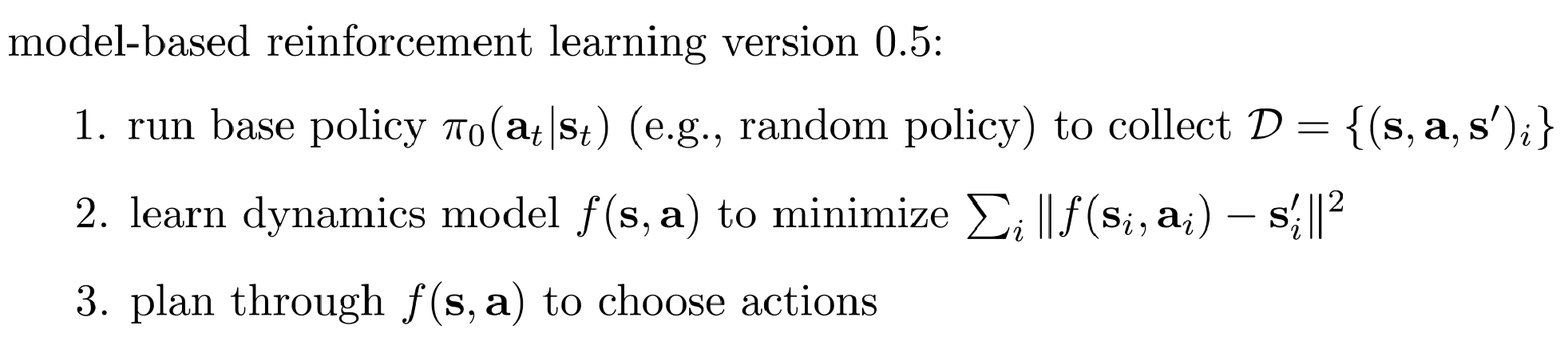
Core Steps
-
One-Time Data Collection
- Collect a static dataset of (state, action, next-state, reward) tuples, typically via random or fixed exploration.
- No further data is gathered afterward.
-
One-Time Model Learning
- Fit a dynamics model \( p_\theta(s' \mid s, a) \) using the static dataset.
- The model may be inaccurate in regions not well-represented in the dataset.
-
One-Time Planning
- Use the learned model to plan or optimize a policy (e.g., via trajectory optimization or tree search).
- The plan is executed in the real environment without re-planning.
Shortcomings
- Distribution Mismatch: The policy can enter states the model has never “seen,” leading to large prediction errors (extrapolation).
- Compounding Errors: Small modeling inaccuracies early on can push the system into unmodeled states, magnifying the errors.
- No Iterative Refinement: With no new data collection, there’s no way to correct model inaccuracies discovered during execution.
Why Move On?
- Severe Mismatch & Error Growth: Because you never adapt to real outcomes beyond the initial dataset, errors can escalate and result in catastrophic failures.
- Limited Practicality: Version 0.5 can work in highly controlled or small problems, but most real tasks require iterative data gathering and model improvements.
Version 1.0: Iterative Re-Fitting + Planning
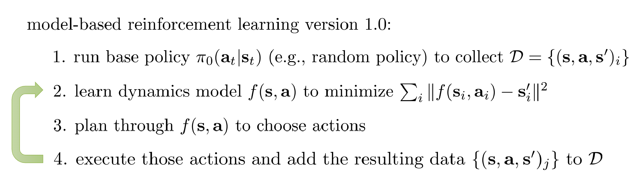
Core Steps
-
Iterative Data Collection
- Use a current policy (or plan) to interact with the environment.
- Gather new transitions (state, action, next-state, reward) and add them to the dataset.
-
Re-Fit the Model
- Update the dynamics model \( p_\theta(s' \mid s, a) \) using the expanded dataset.
- The model gradually learns the dynamics in regions the policy visits.
-
Re-Plan or Update the Policy
- After each model update, re-run planning or policy optimization to refine the policy.
- Deploy the updated policy in the real environment, collect more data, and repeat.
Shortcomings
- Open-Loop Execution: Even though the model is updated iteratively, each plan can be executed “open loop,” so stochastic events or modest model errors can derail a plan until the next re-planning cycle.
- Long-Horizon Vulnerability: If the planning horizon is substantial, inaccuracies can still compound within a single rollout.
Why Move On?
- Stochastic / Complex Tasks: Open-loop plans are brittle. You need a way to correct for real-time deviations instead of waiting until the next iteration.
- Distribution Still Grows: While iterating helps gather more relevant data, you may still face large drifts in states if the environment is noisy or high-dimensional.
Version 1.5: Model Predictive Control (MPC)
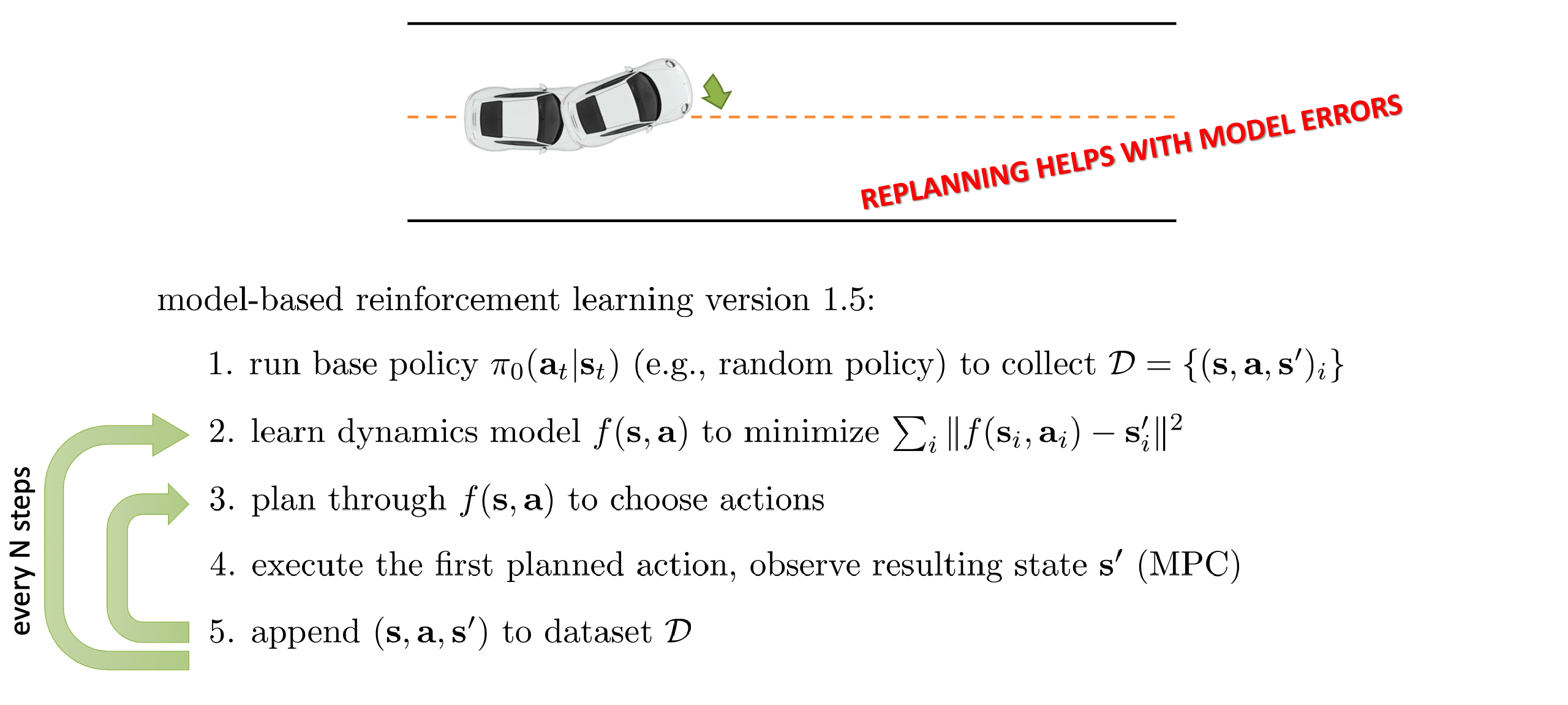
Core Steps
- Short-Horizon Re-Planning at Each Step
-
At each time \(t\):
- Observe the real current state \( s_t \).
- Plan a short sequence of actions \(\{a_t, \dots, a_{t+H-1}\}\) with the learned model.
- Execute only the first action \( a_t \).
- Observe the next real state \( s_{t+1} \).
- Re-plan from \( s_{t+1} \).
-
Closed-Loop Control
-
Frequent re-planning reduces the impact of model errors because the system constantly “checks in” with reality.
-
Iterative Model Updates (Optional)
- As in Version 1.0, you can continue to collect data and update the model periodically.
Shortcomings
- High Computational Cost: Planning at every time step can be expensive, especially in high-dimensional or time-critical domains.
- Still Requires a Good Model: Significant model inaccuracies can still cause erroneous plans, though re-planning mitigates compounding errors.
Why Move On?
- Continuous Planning Overhead: MPC may be infeasible when real-time constraints or massive action spaces make on-the-fly planning too slow.
- Desire for a Learned Policy: A direct policy could yield near-instant action selection at runtime, motivating Version 2.0.
Version 2.0: Backprop Through the Learned Model
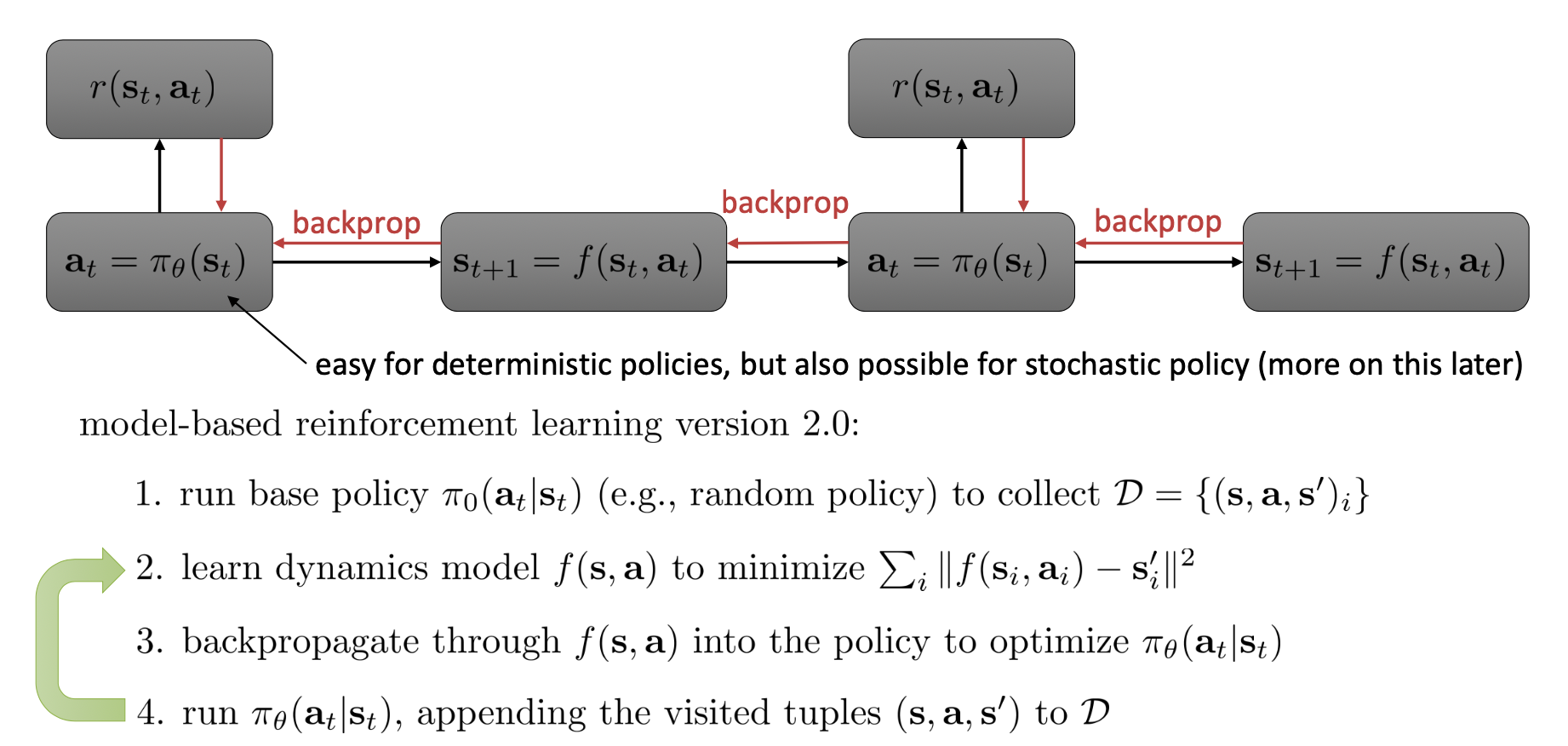
Core Steps
- Differentiable Dynamics Model
-
Train a neural network or another differentiable function \( p_\theta(s' \mid s, a) \).
-
End-to-End Policy Optimization
- Unroll the model over multiple timesteps, applying the policy \(\pi_\phi\) to get actions, and accumulate predicted rewards.
- Backpropagate through the learned model to update policy parameters \(\phi\).
-
Once trained, the resulting policy can be deployed directly—no online planning is needed.
-
High Efficiency at Deployment
- Action selection is a simple forward pass of the policy network, suitable for time-critical or large-scale applications.
Shortcomings
- Numerical Instability: Backpropagating through many timesteps can lead to exploding or vanishing gradients.
- Model Exploitation: The policy can “exploit” any inaccuracies in the model, especially over long horizons or in stochastic environments.
- Careful Regularization: Shorter horizon unrolls, ensembles, or uncertainty estimation are often used to keep policy learning stable and robust.
Why Move On?
Well, Version 2.0 is often seen as an “end goal” rather than a stepping stone—because once you have a learned policy that requires no online planning, you enjoy high-speed inference. However: - Complexity and Instability: Real-world tasks may need a mix of methods (e.g., partial MPC, ensembles) to handle uncertainty and prevent exploitation of model errors.
Reward Overshooting (Overoptimistic Planning)
What It Is
- Definition: When a planner or policy exploits incorrect or extrapolated high reward predictions from the learned model, leading to unrealistic or unsafe behavior in the real environment.
Why It Happens
- Sparse Coverage: The model has little data in certain regions, so it overestimates rewards there.
- Open-Loop Plans: Versions 0.5 and 1.0 may chase these “fantasy” states for an entire rollout before correcting in the next iteration.
- Uncertainty Blindness: If the approach doesn’t penalize states with high model uncertainty, the planner may favor them solely because the model “thinks” they are high-reward.
Consequences
- Poor Real-World Transfer: The agent’s performance can appear great under the learned model but fail in actual interaction.
- Safety Violations: In real-world robotics or critical applications, overshooting can lead to dangerous actions.
Mitigation Strategies
- Frequent Re-Planning (MPC): Correct for erroneous predictions step by step.
- Iterative Data Collection: Gradually gather real data in uncertain regions.
- Uncertainty-Aware Models: Ensembles or Bayesian approaches that identify high-uncertainty states and penalize them.
- Regularization: Shorter horizon rollouts, trust regions, or other constraints limit destructive exploitation of model errors.
Other Challenges and Notes
-
Reward Function Misspecification. If the reward function itself is imperfect or learned, it can exacerbate overshooting or produce unintended behaviors.
-
Stochastic Environments. Open-loop methods (Version 0.5, 1.0) can fail if they don’t adapt in real time. MPC (Version 1.5) or robust policy optimization (Version 2.0) are better at handling randomness.
-
Exploding/Vanishing Gradients. A big challenge for Version 2.0 when unrolling many timesteps through a neural model.
-
Safety Concerns. In physical or high-stakes domains, any form of model inaccuracy can be dangerous. MPC is often the pragmatic choice in safety-critical tasks.
-
Computational Trade-Offs. MPC (Version 1.5) can be expensive online. End-to-end policy learning (Version 2.0) moves the heavy lifting offline, but training is more delicate.
5. Dynamics Model Learning
Learning a model \(\hat{P}(s_{t+1}\mid s_t,a_t)\) + \(\hat{R}(s_t,a_t)\) is often done via supervised learning on transitions \((s_t,a_t,s_{t+1},r_t)\). This section surveys advanced considerations from Moerland et al. .
5.1 Basic Considerations
-
Type of Model
- Forward (most common): \((s_t,a_t)\mapsto s_{t+1}\).
- Backward (reverse model): \(s_{t+1}\mapsto (s_t,a_t)\). Used in prioritized sweeping.
- Inverse: \((s_t, s_{t+1}) \mapsto a_t\). Sometimes used in representation learning or feedback control.
-
Estimation Method
- Parametric (e.g., neural networks, linear regressors, GPs).
- Non-parametric (e.g., nearest neighbors, kernel methods).
- Exact (tabular) vs. approximate (function approximation).
-
Region of Validity
- Global model: Attempt to capture all states. Common in large-scale MBRL.
- Local model: Fit only around the current trajectory or region of interest (common in robotics, e.g., local linearization).
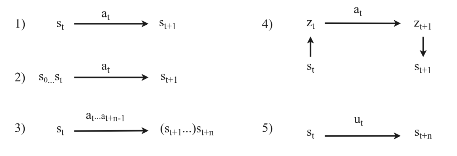 Overview of different types of mappings in model learning. 1) Standard Markovian transition model \( s_t, a_t \rightarrow s_{t+1} \). 2) Partial observability. We model \( s_0 \ldots s_t, a_t \rightarrow s_{t+1} \), leveraging the state history to make an accurate prediction. 3) Multi-step prediction (Section 4.6), where we model \( s_t, a_t \ldots a_{t+n-1} \rightarrow s_{t+n} \), to predict the \( n \) step effect of a sequence of actions. 4) State abstraction, where we compress the state into a compact representation \( z_t \) and model the transition in this latent space. 5) Temporal/action abstraction, better known as hierarchical reinforcement learning, where we learn an abstract action \( u_t \) that brings us to \( s_{t+n} \). Temporal abstraction directly implies multi-step prediction, as otherwise the abstract action \( u_t \) is equal to the low level action \( a_t \). All the above ideas (2–5) are orthogonal and can be combined.
5.2 Stochasticity
Real MDPs can be stochastic, meaning that the environment transition from \((s_t, a_t)\) to \(s_{t+1}\) is governed by a distribution:
Unlike a deterministic setting (where we might write \(s_{t+1} = f(s_t, a_t)\)), this transition function yields a probability distribution over all possible next states rather than a single outcome.
5.2.1 Multi-Modal Transitions and the Conditional Mean Problem
When training a purely deterministic network (e.g., a standard neural network with mean-squared error, MSE) to predict \(s_{t+1}\) from \((s_t, a_t)\), the model typically learns the conditional mean of the next-state distribution. This can be problematic if the true transition distribution is multi-modal, since the mean might not align with any actual or likely realization of the environment.
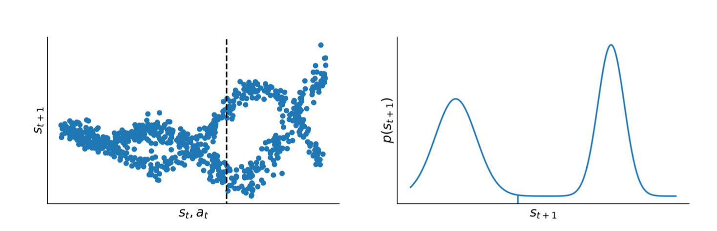
Illustration of stochastic transition dynamics. Left: 500 samples from an example transition function \(P(s_{t+1} \mid s, a)\). The vertical dashed line indicates the cross-section distribution on the right. Right: distribution of \(s_{t+1}\) for a particular \((s, a)\). We observe a multimodal distribution. The conditional mean of this distribution, which would be predicted by MSE training, is shown as a vertical line.
Formally, if the true next state is a random variable \(S_{t+1}\), then MSE-based regression gives
Hence, if \(S_{t+1}\) can take on several distinct modes with similar probabilities, a single mean prediction \(\hat{s}_{t+1}\) may not capture the actual modes at all.
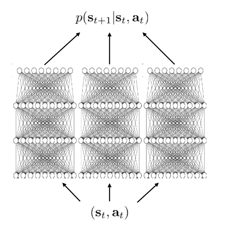
5.2.2 Descriptive (Distribution) Models
To capture multi-modal dynamics rigorously, one can represent the full distribution \(P(s_{t+1}\mid s_t,a_t)\). Common choices include:
-
Gaussian Distribution
Assume\[ s_{t+1} \;\sim\; \mathcal{N}\bigl(\mu_\theta(s_t,a_t),\,\Sigma_\theta(s_t,a_t)\bigr), \]where \(\theta\) denotes model parameters. Typically trained by maximizing log-likelihood of observed transitions.
-
Gaussian Mixture Models (GMM)
Use a sum of \(K\) Gaussians:\[ s_{t+1} \;\sim\; \sum_{k=1}^{K}\;\alpha_k(\theta; s_t,a_t)\;\mathcal{N}\!\Bigl(\mu_k,\;\Sigma_k\Bigr). \]The mixture weights \(\alpha_k\) sum to 1. This better captures multi-modality than a single Gaussian but can be more complex to train (e.g., via EM).
-
Tabular/Histogram-Based
For lower-dimensional or discrete states:\[ \hat{P}\bigl(s' \mid s,a\bigr) \;=\; \frac{n(s,a,s')}{\sum_{\tilde{s}}\,n(s,a,\tilde{s})}, \]where \(n(\cdot)\) counts observed transitions. This is often infeasible in large or continuous domains.
5.2.3 Generative Approaches
Instead of closed-form probability distributions, one might learn a generative mapping that samples from \(P(s_{t+1}\mid s_t,a_t)\). Examples:
-
Variational Autoencoders (VAEs)
Introduce a latent variable \(\mathbf{z}\). Then\[ s_{t+1} \;=\; f_\theta\!\bigl(\mathbf{z},\,s_t,\,a_t\bigr), \quad \mathbf{z}\;\sim\;\mathcal{N}(\mathbf{0},\mathbf{I}), \]and fit \(\theta\) via variational inference. Inference-time sampling of \(\mathbf{z}\) yields diverse future states.
-
Normalizing Flows
Transform a simple base distribution (like a Gaussian) through a stack of invertible mappings \(\{f_\theta^{(\ell)}\}\):\[ \mathbf{z}\,\sim\,\mathcal{N}(\mathbf{0},\mathbf{I}), \quad s_{t+1} \;=\; (f_\theta^{(L)} \circ \cdots \circ f_\theta^{(1)})(\mathbf{z}). \]Optimized via maximum likelihood, enabling expressive densities.
-
Generative Adversarial Networks (GANs)
A discriminator \(D\) distinguishes real vs. generated next states, while the generator \(G\) attempts to fool \(D\). Though flexible, GAN training can be unstable or prone to mode collapse. -
Autoregressive Models
Factorize high-dimensional \(s_{t+1}\) into a chain of conditionals. Useful for image-based transitions but can be computationally heavy.
5.2.4 Training Objectives
Most distribution models are trained by maximizing likelihood or minimizing negative log-likelihood over a dataset \(\{(s_t^{(i)}, a_t^{(i)}, s_{t+1}^{(i)})\}\). For example:
where \(\Omega(\theta)\) might be a regularization term. GAN-based models use a min-max objective, while VAE-based methods use an ELBO that includes a reconstruction term and a KL prior penalty on the latent space.
5.2.5 Practical Considerations and Challenges
-
Divergence in Multi-Step Rollouts
Even with a stochastic model, errors can accumulate as predictions are fed back into the model. Mitigations include unrolling during training, multi-step loss functions, or specialized architectures. -
Mode Collapse / Rare Transitions
Multi-modal distributions can be hard to learn in practice. Models must capture all critical modes, especially for safety or robotics contexts where minority transitions may be crucial. -
High-Dimensional Observations
Image-based tasks often leverage latent-variable models (e.g., VAE-like) to reduce dimensionality. Encoding \(\rightarrow\) (predict in latent space) \(\rightarrow\) decoding is common. -
Expressiveness vs. Efficiency
Complex generative models (e.g., large mixtures or flows) capture stochasticity better but are often slower to train and evaluate. Many real-world agents resort to simpler unimodal Gaussians, balancing speed and accuracy.
5.2.6 Example: Gaussian Transitions via Maximum Likelihood
A common assumption uses a unimodal Gaussian:
Assume diagonal covariance \(\Sigma_\theta=\mathrm{diag}(\sigma_1^2,\dots,\sigma_d^2)\). The log-likelihood for one observed transition is:
Maximizing this finds a Gaussian best-fit to the empirical data. While unimodal, it remains a popular, tractable choice for continuous control.
5.2.7 Concluding Remarks on Stochastic Transitions
-
Why Model Stochasticity?
Real-world dynamics often have multiple plausible next states. Failing to capture these can produce inaccurate planning and suboptimal policies. -
Descriptive vs. Generative
Some tasks demand full density estimation (e.g., risk-sensitive planning), while others only require sampling plausible transitions (e.g., for Monte Carlo rollouts). -
Integration with RL
Once a model is learned, the agent can plan by either averaging over transitions or sampling them. Handling many branching futures can be computationally expensive; practical approaches limit the depth or use heuristic expansions.
In sum, real-world MDPs often present multi-modal and stochastic dynamics. A purely deterministic predictor trained via MSE collapses the distribution to a single mean. Instead, we can use distribution (e.g., GMM) or generative (e.g., VAE, flows, GANs) approaches, trained via maximum likelihood, adversarial losses, or variational inference. Proper handling of stochastic transitions is essential for robust planning, policy optimization, and multi-step simulation in model-based RL.
5.3 Uncertainty
A critical challenge in MBRL is model uncertainty—the model is learned from limited data, so predictions can be unreliable in unfamiliar state-action regions. We distinguish:
- Aleatoric (intrinsic) uncertainty: inherent stochasticity in transitions.
- Epistemic (model) uncertainty: arises from limited training data. This can, in principle, be reduced by gathering more data.
A rigorous approach is to maintain a distribution over possible models, then plan by integrating or sampling from that distribution to avoid catastrophic exploitation of untrusted model regions.
Bayesian Neural Networks
One approach is a Bayesian neural network (BNN):
We keep a posterior \(p(\theta\mid D)\) over network weights \(\theta\) given dataset \(D\). Predictive distribution for the next state is then:
In practice, approximations like variational dropout or Laplace approximation are used to sample from \(p(\theta)\).
Ensembles and Bootstrapping
Another popular method is an ensemble of \(N\) models \(\{\hat{P}_{\theta_i}\}\). Each model is trained on a bootstrapped subset of the data (or with different initialization seeds). The variance across predictions:
indicates epistemic uncertainty. In practice:
During planning, one may:
- Sample one model from the ensemble at each step (like PETS).
- Average the predictions or treat it as a Gaussian mixture model.
Either way, uncertain regions typically manifest as a large disagreement among ensemble members, warning the planner not to trust that zone.
Mathematically: if the “true” dynamics distribution is \(P^\star\) and each model \(\hat{P}_{\theta_i}\) is an unbiased estimator, then large variance across \(\{\hat{P}_{\theta_i}\}\) signals a region outside the training distribution. Minimizing that variance can guide exploration or help shape conservative planning.
5.4 Partial Observability
Sometimes the environment is not fully observable. We can’t identify the full state \(s\) from a single observation \(o\). Solutions:
- Windowing: Keep last \(n\) observations \((o_t, o_{t-1}, \dots)\).
- Belief state: Use a hidden Markov model or Bayesian filter.
- Recurrence: Use RNNs/LSTMs that carry hidden state \(\mathbf{h}_t\).
- External Memory: Neural Turing Machines, etc., for long-range dependencies.
5.5 Non-Stationarity
Non-stationary dynamics means that \(P\) or \(R\) changes over time. A single learned model can become stale. Approaches include:
- Partial models [Doya et al., 2002]: Maintain multiple submodels for different regimes, detect changes in transition error.
- High learning-rate or forgetting older data to adapt quickly.
5.6 Multi-Step Prediction
One-step predictions can accumulate error when rolled out repeatedly. Some solutions:
- Train for multi-step: Unroll predictions for \(k\) steps and backprop against ground truth \((s_{t+k})\).
- Dedicated multi-step models: Instead of chaining one-step predictions, learn \(f^{(k)}(s_t,a_{t:k-1})\approx s_{t+k}\).
5.7 State Abstraction
In many domains, the raw observation space \(s\) can be very high-dimensional (e.g., pixel arrays), making direct modeling of \((s_t, a_t) \mapsto s_{t+1}\) intractable. State abstraction (or representation learning) tackles this issue by learning a more compact latent state \(\mathbf{z}_t\), capturing the essential factors of variation. Once in this latent space, the model learns transitions \(\mathbf{z}_{t+1} = f_{\text{trans}}(\mathbf{z}_t, a_t)\), and can decode back to the original space if needed:
This structure reduces modeling complexity and can enable more efficient planning or control in the latent domain.
5.7.1 Common Approaches to Representation Learning
-
Autoencoders and Variational Autoencoders (VAEs)
An autoencoder aims to learn an encoding \(\mathbf{z}=f_{\text{enc}}(s)\) that, when passed through a decoder \(f_{\text{dec}}\), reconstructs the original state \(s\). In variational autoencoders (VAEs), one imposes a prior distribution \(p(\mathbf{z})\) (often Gaussian) over the latent space, adding a Kullback–Leibler (KL) divergence penalty:\[ \max_{\theta,\phi} \;\; \mathbb{E}_{q_\phi(\mathbf{z}\mid s)} \Bigl[\log p_\theta(s\mid \mathbf{z})\Bigr] \;-\; D_{\mathrm{KL}}\bigl(q_\phi(\mathbf{z}\mid s)\,\|\,p(\mathbf{z})\bigr), \]where \(q_\phi(\mathbf{z}\mid s)\) is the encoder distribution and \(p_\theta(s\mid \mathbf{z})\) is the decoder. This ensures the learned latent code \(\mathbf{z}\) both reconstructs well and remains “organized” under the prior \(p(\mathbf{z})\). Once learned, a latent dynamics model \(\mathbf{z}_{t+1}=f_{\text{trans}}(\mathbf{z}_t,a_t)\) can be fitted by minimizing a prediction loss (e.g., mean-squared error on \(\mathbf{z}\)-space).
-
Object-Based Approaches
For environments that can be factorized into distinct objects (e.g., multiple physical entities), Graph Neural Networks (GNNs) or object-centric models can more naturally capture the underlying structure. Concretely, each latent node \(\mathbf{z}_i\) corresponds to an object’s state (e.g., location, velocity, shape), and edges model interactions among objects. Formally,\[ \mathbf{z}_{t+1}^{(i)} \;=\; f_{\text{trans}}^{(i)} \Bigl( \mathbf{z}_t^{(i)},\,a_t,\, \{\mathbf{z}_t^{(j)}\}_{j \in \mathcal{N}(i)} \Bigr), \]where \(\mathcal{N}(i)\) denotes neighbors of object \(i\). This is particularly effective in physics-based settings [Battaglia et al., 2016], allowing each object’s transition to depend primarily on relevant neighbors (e.g., collisions). Such structured representations often facilitate better generalization to new configurations (e.g., changing the number or arrangement of objects).
-
Contrastive Losses for Semantic/Controllable Features
Sometimes, a purely reconstruction-based loss can over-focus on visually salient but decision-irrelevant details. Contrastive methods use pairs (or triplets) of observations to emphasize meaningful relationships. For instance, if two states \(s\) and \(s'\) are known to be dynamically close (reachable with few actions), one encourages their embeddings \(\mathbf{z}\) and \(\mathbf{z}'\) to be close under some metric. Formally, a contrastive loss might look like:\[ \ell_{\mathrm{contrast}}(\mathbf{z}, \mathbf{z}') \;=\; y\,\|\mathbf{z}-\mathbf{z}'\|^2 \;+\; (1-y)\,\bigl[\alpha - \|\mathbf{z}-\mathbf{z}'\|\bigr]_{+}, \]where \(y=1\) if the states should be similar, and \(y=0\) otherwise, and \(\alpha\) is a margin. Examples include time-contrastive approaches [Sermanet et al., 2018] that bring together frames from different camera angles but the same physical scene, or goal-oriented distances [Ghosh et al., 2018]. These tasks guide the learned \(\mathbf{z}\)-space to capture features that matter for control, rather than trivial background details.
5.7.2 Planning in Latent Space
Once a latent representation is established, an agent can:
-
Plan directly in \(\mathbf{z}\)-space
For instance, run a forward-search or gradient-based policy optimization with states \(\mathbf{z}\) and transitions \(f_{\text{trans}}(\mathbf{z}, a)\). If the decoder \(f_{\text{dec}}\) is not explicitly needed (e.g., if the agent only needs to output actions), planning in the latent domain can reduce computational overhead and reduce the “curse of dimensionality.” -
Decode for interpretability or environment feedback
If the environment requires real-world actions or if interpretability is desired, one can decode predicted latent states \(\mathbf{z}_{t+1}\) to \(\hat{s}_{t+1}\). The environment then checks feasibility or yields a reward. This is especially relevant when the environment is external (like a simulator or the real world) expecting inputs in the original space.
A primary challenge is rollout mismatch: if \(\mathbf{z}_{t+1}\) is never trained to match \(f_{\text{enc}}(s_{t+1})\), repeated application of \(f_{\text{trans}}\) might accumulate errors. Solutions include explicit consistency constraints (i.e., \(\|\mathbf{z}_{t+1} - f_{\text{enc}}(s_{t+1})\|\) penalties) or probabilistic latent inference (e.g., Kalman filter variants, sequential VAEs).
5.8 Temporal Abstraction
In Markov Decision Processes (MDPs), each action typically spans one environment step. But many tasks have natural subroutines that can be chunked into higher-level actions. This is the essence of hierarchical reinforcement learning (HRL): define “macro-actions” that unfold over multiple timesteps, reducing effective planning depth and often improving data efficiency.
5.8.1 Options Framework
An Option \(\omega\) is a tuple \((I_\omega, \pi_\omega, \beta_\omega)\) [Sutton et al., 1999]:
- Initiation set \(I_\omega \subseteq \mathcal{S}\): states from which \(\omega\) can be invoked.
- Subpolicy \(\pi_\omega(a \mid s)\): governs low-level actions while the option runs.
- Termination condition \(\beta_\omega(s)\): probability that \(\omega\) terminates upon reaching state \(s\).
When executing option \(\omega\), the agent follows \(\pi_\omega\) until a stochastic termination event triggers, transitioning back to the high-level policy’s control. The high-level policy thus selects from a set of options, each a multi-step “chunk” of actions. This can drastically reduce the horizon of the planning problem.
Mathematically, a semi-MDP formalism captures these temporally extended actions, where option \(\omega\) yields a multi-step transition \((s, \omega)\mapsto s'\). One can learn option-value functions \(Q(s,\omega)\) or plan with pseudo-rewards inside each option. In practice, good options can significantly accelerate learning and planning compared to primitive actions.
5.8.2 Goal-Conditioned Policies
Alternatively, goal-conditioned or universal value functions [Schaul et al., 2015] define a function \(Q(s, a, g)\) that specifies the expected return for taking action \(a\) in state \(s\) while aiming to achieve goal \(g\). One can then plan by selecting subgoals:
where each “macro-step” is the agent trying to reach \(g_i\) from the current state. Feudal RL frameworks [Dayan and Hinton, 1993] similarly treat higher-level “managers” that set subgoals for lower-level “workers.” A learned, goal-conditioned subpolicy \(\pi(a\mid s,g)\) can generalize across different goals \(g\), unlike the options approach that typically uses separate subpolicies per option.
5.8.3 Subgoal Discovery
A key research question is how to discover effective macro-actions (options) or subgoals. Approaches include:
-
Graph-based Bottlenecks
Construct or approximate a graph of states/regions. Identify bottlenecks as states that connect densely connected regions. Formally, if a state \(s\) lies on many shortest paths between subregions of the state space, it can be a strategic “bridge.” Setting it as a subgoal can simplify global planning [Menache et al., 2002]. -
Empowerment / Coverage
Encourage subpolicies that cover different parts of the state space or yield high controllability. For instance, one might maximize mutual information between subpolicy latent codes and resulting states, ensuring distinct subpolicies lead to distinct outcomes. This fosters diverse skill discovery. -
End-to-End Learning
Methods like Option-Critic [Bacon et al., 2017] embed option structure into a differentiable policy architecture and optimize for return. The subpolicies and termination functions emerge from gradient-based training, though careful regularization is often needed to avoid degenerate solutions (e.g., a single subpolicy doing everything).
5.8.4 Benefits of Temporal Abstraction
- Reduced Planning Depth
Since each macro-action can span multiple timesteps, the effective decision horizon shrinks, often simplifying search or dynamic programming. - Transfer and Reuse
Once discovered, options/subpolicies can be reused in related tasks. If those subroutines correspond to meaningful skills, the agent may quickly adapt to new goals. - Data Efficiency
Higher-level actions can yield more stable and purposeful exploration, collecting relevant experience faster than random primitive actions.
6. Integration of Planning and Learning
With a learned model in hand (or a known one), we combine planning and learning to optimize a policy \(\pi\). We address four major questions:
- Which state to start planning from?
- Budget and frequency: how many real steps vs. planning steps?
- Planning algorithm: forward search, MCTS, gradient-based, etc.
- Integration: how planning outputs feed into policy/value updates and final action selection.
6.1 Which State to Start Planning From?
- Uniform over all states (like classical dynamic programming).
- Visited states only (like Dyna [Sutton, 1990], which samples from replay).
- Prioritized (Prioritized Sweeping [Moore & Atkeson, 1993]) if some states need urgent update.
- Current state only (common in online MPC or MCTS from the real agent’s state).
6.2 Planning Budget vs. Real Data Collection
Two sub-questions:
-
Frequency: plan after every environment step, or collect entire episodes first?
- Dyna plans after each step (like 100 imaginary updates per real step).
- PILCO [Deisenroth & Rasmussen, 2011] fits a GP model after each episode.
-
Budget: how many model rollouts or expansions per planning cycle?
- Dyna might do 100 short rollouts.
- AlphaZero expands a single MCTS iteration by up to 1600 × depth calls.
Some methods adaptively adjust planning vs. real data based on model uncertainty [Kalweit & Boedecker, 2017]. The right ratio can significantly affect performance.
6.3 How to Plan? (Planning Algorithms)
Broadly:
-
Discrete (non-differentiable) search:
- One-step lookahead
- Tree search (MCTS, minimax)
- Forward vs. backward: e.g., prioritized sweeping uses a reverse model to propagate value changes quickly
-
Differential (gradient-based) planning:
- Requires a differentiable model \(\hat{P}\).
- E.g., iterative LQR, or direct backprop through unrolled transitions (Dreamer).
- Suited for continuous control with smooth dynamics.
-
Depth & Breadth choices:
- Some do short-horizon expansions (MBPO uses 1–5 step imaginary rollouts).
- Others do deeper expansions if computing resources allow (AlphaZero MCTS).
-
Uncertainty handling:
- Plan only near states with low model uncertainty or penalize uncertain states.
- Ensemble-based expansions [Chua et al., 2018].
Cross-Entropy Method (CEM) – Pseudocode
    # Suppose we want to find the best action sequence of length H
    # that maximizes the expected return under our model.

    Initialize distribution params (mean mu, covariance Sigma)
    for iteration in range(N_iterations):
        # 1. Sample K sequences from current distribution
        candidate_sequences = sample_from_gaussian(mu, Sigma, K)

        # 2. Evaluate each sequence's return
        returns = []
        for seq in candidate_sequences:
            returns.append( evaluate_return(seq, model) )

        # 3. Select the top M (elite) sequences
        elite_indices = top_indices(returns, M)
        elites = [candidate_sequences[i] for i in elite_indices]

        # 4. Update mu, Sigma to fit the elites
        mu = mean(elites)
        Sigma = cov(elites)

    # Final distribution reflects the best action sequence
    best_action_seq = mu
    return best_action_seq
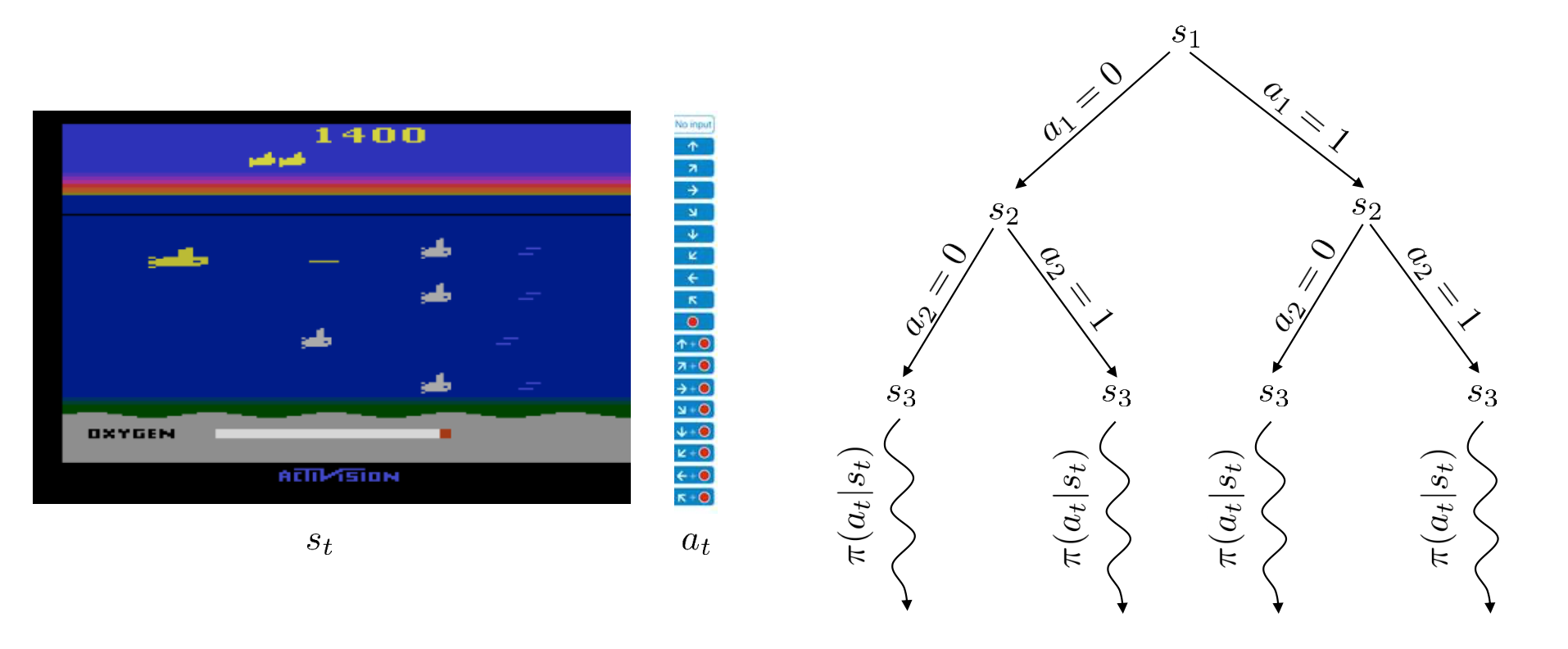
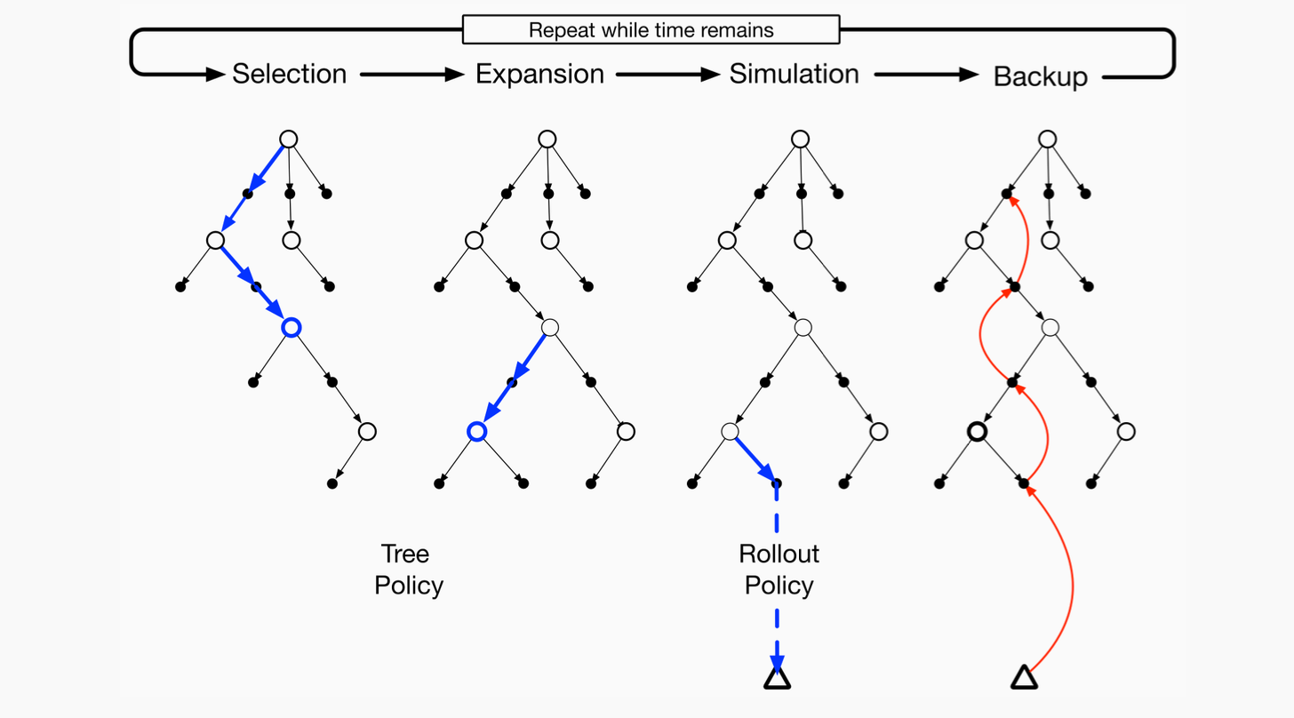
6.3.1 Monte Carlo Tree Search (MCTS)
Monte Carlo Tree Search is a powerful method for discrete action planning—famously used in AlphaGo, AlphaZero, MuZero. Key components:
-
Tree Representation
- Each node is a state, edges correspond to actions.
- MCTS incrementally expands the search tree from a root (the current state).
-
Four Steps commonly described as:
- Selection: Repeatedly choose child nodes (actions) from the root, typically via Upper Confidence Bound or policy heuristics, until reaching a leaf node.
- Expansion: If the leaf is not terminal (or at max depth), add one or more child nodes for possible next actions.
- Simulation: From that new node, simulate a rollout (random or policy-driven) until reaching a terminal state or horizon.
- Backpropagation: Propagate the return from the simulation up the tree to update value/statistics at each node.
-
Mathematical Form
- Let \(N(s,a)\) be the number of visits to child action \(a\) from state \(s\).
- Let \(\hat{Q}(s,a)\) be the estimated action-value from MCTS.
-
UCB selection uses:
\[ a_\text{select} = \arg\max_{a}\Bigl[\hat{Q}(s,a) + c \sqrt{\frac{\ln \sum_{b} N(s,b)}{N(s,a)}}\Bigr]. \](One can also incorporate a learned prior policy \(\pi_\theta\) to bias exploration.)
-
Planning & Policy Extraction
- After many simulations from the root, MCTS typically normalizes node visits or Q-values to produce a final policy distribution \(\alpha\).
- This policy \(\alpha\) may be used for real action selection, or to train a global policy network (as in AlphaZero).
MCTS Pseudocode
MCTS(root_state, model, N_simulations)
Initialize the search tree with root_state

for simulation in 1 to N_simulations do
    node ← root of the tree

    # Selection
    while node is fully expanded and node is not terminal do
        action ← select child of node using UCB
        node ← child corresponding to action

    # Expansion
    if node is not terminal then
        expand node using model (generate all children)
        node ← select one of the new children

    # Simulation
    reward ← simulate from node.state using model

    # Backpropagation
    backpropagate reward up the tree from node

# Final decision
Return action from root with highest visit count
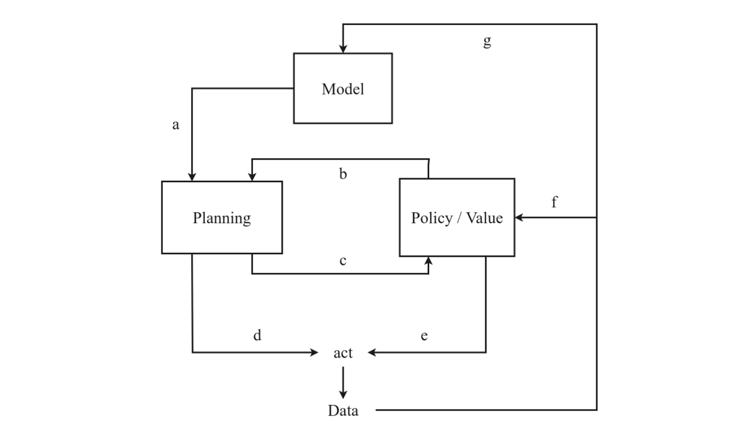
6.4 Integration in the Learning and Acting Loop
Key integration channels:
-
Planning input from existing policy/value?
- E.g., MCTS uses a prior policy to guide expansions.
-
Planning output as a training target for the global policy/value?
- E.g., Dyna uses imaginary transitions to update Q-values.
- AlphaZero uses MCTS results as a learning target for \(\pi\) and \(V\).
-
Action selection from the planning procedure or from the learned policy?
- E.g., MPC picks the best action from a planned sequence.
- Or a final learned policy is used if no real-time planning is feasible.
Various combinations exist: some methods rely mostly on the learned policy but refine or correct it with a short replan (MBPO), while others do a full MCTS at every step (MuZero).
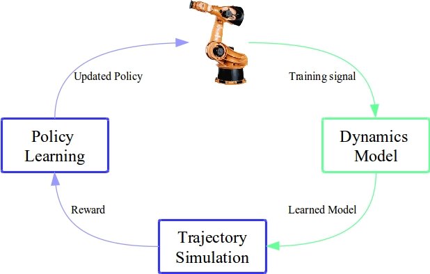
6.5 Dyna and Dyna-Style Methods
One of the earliest and most influential frameworks for model-based RL is Dyna [Sutton, 1990]. The key insight is to integrate:
- Real experience from the environment (sampled transitions)
- Model learning from that real data
- Imagined experience from the learned model to augment the policy/value updates.
Dyna Pseudocode
Input: α (learning rate), γ (discount factor), ε (exploration rate),
       n (number of planning steps), num_episodes

Initialize Q(s, a) arbitrarily for all states s ∈ S, actions a ∈ A
Initialize Model as an empty mapping: Model(s, a) → (r, s')

for each episode do
    Initialize state s ← starting state

    while s is not terminal do
        ▸ Action Selection (ε-greedy)
        With probability ε: choose random action a
        Else: choose a ← argmax_a Q(s, a)

        ▸ Real Interaction
        Take action a, observe reward r and next state s'

        ▸ Q-Learning Update
        Q(s, a) ← Q(s, a) + α [ r + γ · max_a' Q(s', a') − Q(s, a) ]

        ▸ Model Update
        Model(s, a) ← (r, s')

        ▸ Planning (n simulated updates)
        for i = 1 to n do
            Randomly select previously seen (ŝ, â)
            (r̂, ŝ') ← Model(ŝ, â)

            Q(ŝ, â) ← Q(ŝ, â) + α [ r̂ + γ · max_a' Q(ŝ', a') − Q(ŝ, â) ]

        ▸ Move to next real state
        s ← s'
- Real Interaction: We pick action \(a\) in state \(s\) using \(\epsilon\)-greedy w.r.t. \(Q\).
- Update Q from real transition \((s,a,s',r)\).
- Update Model: store or learn to predict \(\hat{P}(s'\mid s,a)\), \(\hat{R}(s,a)\).
- Imagination (N_planning steps): randomly sample a state-action pair from replay or memory, query the model for \(\hat{s}', \hat{r}\). Update \(Q\) with that synthetic transition.
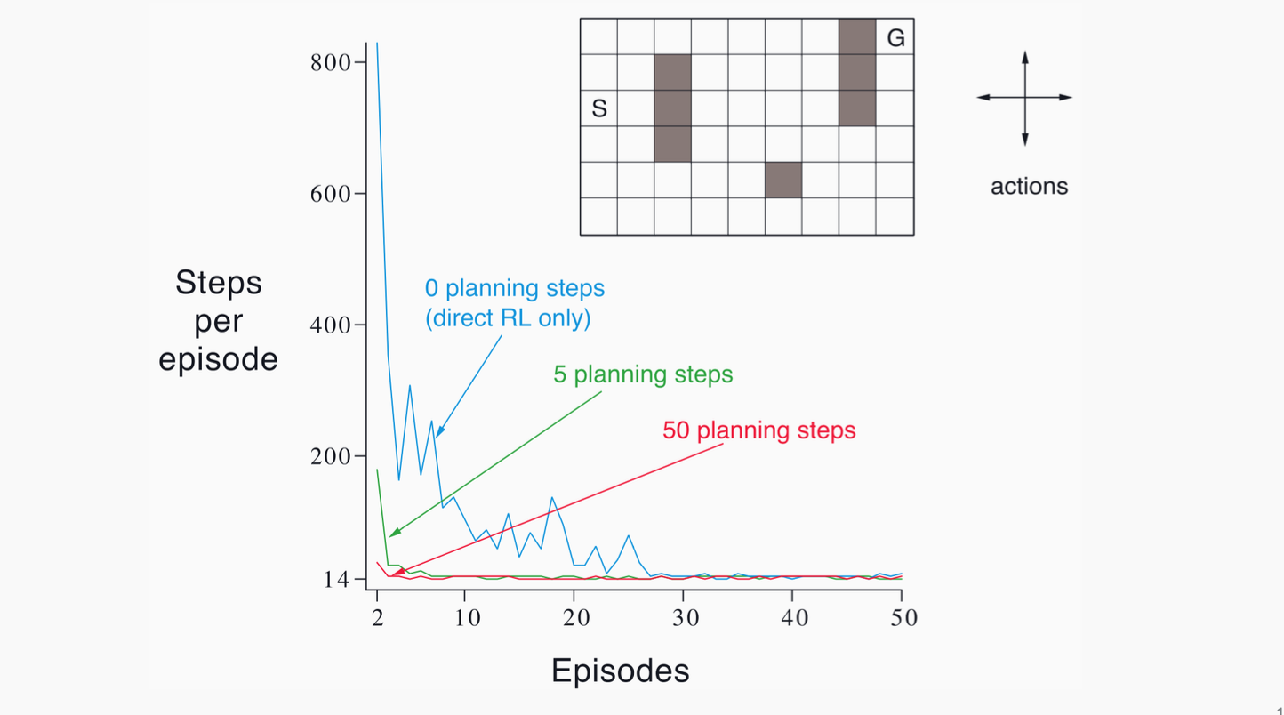
Benefits:
- Dyna can drastically reduce real environment interactions by effectively replaying or generating new transitions from the learned model.
- Even short rollouts or repeated “one-step planning” from random visited states helps refine Q-values more quickly.
Dyna-Style in modern deep RL:
- Many algorithms (e.g., MBPO) add short-horizon imaginary transitions to an off-policy buffer.
- They differ in details: how many model steps, how they sample states for imagination, how they manage uncertainty, etc.
7. Modern Model-Based RL Algorithms
Modern model-based RL builds on classical ideas (global/local models, MPC, iterative re-fitting) but incorporates powerful neural representations, uncertainty handling, and integrated planning-learning frameworks. Below are five influential algorithms that illustrate the state of the art in contemporary MBRL.
7.1 World Models (Ha & Schmidhuber, 2018)
Core Idea
Train a latent generative model of the environment (specifically from high-dimensional inputs like images), and then learn or optimize a policy entirely within this learned latent space—the so-called “dream environment.”
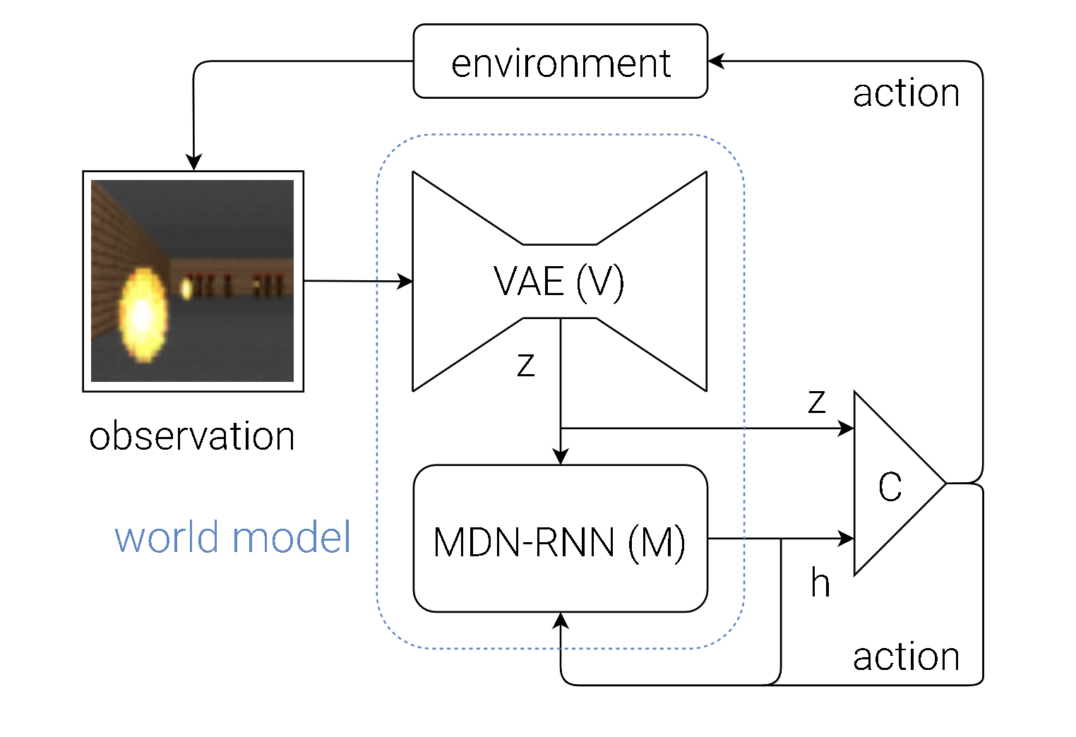
Key Components
-
Variational Autoencoder (VAE):
- Maps raw observation \(\mathbf{o}_t\) to a compact latent representation \(\mathbf{z}_t\).
- \(\mathbf{z}_t = E_\phi(\mathbf{o}_t)\) where \(E_\phi\) is the learned encoder.
- Reconstruction loss ensures \(E_\phi\) and a corresponding decoder \(D_\phi\) compress and reconstruct images effectively.
-
Recurrent Dynamics Model (MDN-RNN):
- Predicts the next latent \(\mathbf{z}_{t+1}\) given \(\mathbf{z}_t\) and action \(a_t\).
-
Often parameterized as a Mixture Density Network inside an RNN:
\[ \mathbf{z}_{t+1} \sim p_\theta(\mathbf{z}_{t+1} \mid \mathbf{z}_t, a_t). \] -
This distribution can be modeled by a mixture of Gaussians, providing a probabilistic estimate of the next latent state.
-
Controller (Policy):
- A small neural network \(\pi_\eta\) that outputs actions \(a_t = \pi_\eta(\mathbf{z}_t)\) in the latent space.
- Trained (in the original paper) via an evolutionary strategy (e.g., CMA-ES) entirely in the dream world.
Algorithmic Flow
- Unsupervised Phase: Run a random or exploratory policy in the real environment, collect observations \(\mathbf{o}_1, \mathbf{o}_2, ...\).
- Train the VAE to learn \(\mathbf{z} = E_\phi(\mathbf{o})\).
- Train the MDN-RNN on sequences \((\mathbf{z}_t, a_t, \mathbf{z}_{t+1})\).
- “Dream”: Roll out the MDN-RNN from random latents and evaluate candidate controllers \(\pi_\eta\).
- Update \(\pi_\eta\) based on the dream performance (e.g., via evolutionary search).
Significance
- Demonstrated that an agent can learn a world model of high-dimensional environments (CarRacing, VizDoom) and train policies in “latent imagination.”
- Paved the way for subsequent latent-space MBRL (PlaNet, Dreamer).
7.2 PETS (Chua et al., 2018)
Core Idea
Probabilistic Ensembles with Trajectory Sampling (PETS) uses ensemble neural network dynamics models to capture epistemic uncertainty, combined with sampling-based planning (like the Cross-Entropy Method, CEM) for continuous control.
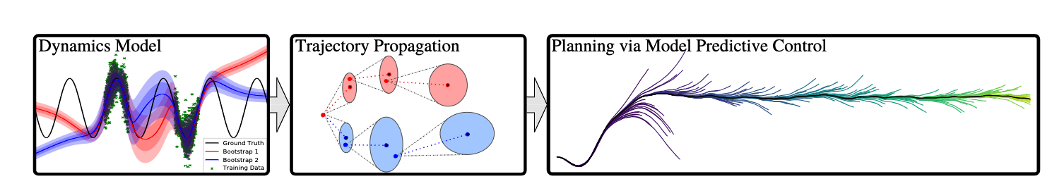
Modeling Uncertainty
- Train \(N\) distinct neural networks \(\{\hat{P}_{\theta_i}\}\), each predicting \(\mathbf{s}_{t+1}\) given \(\mathbf{s}_t, a_t\).
- Each network outputs a mean \(\mathbf{\mu}_i\) and variance \(\mathbf{\Sigma}_i\) for \(\mathbf{s}_{t+1}\).
- Ensemble Disagreement can signal model uncertainty, guiding more cautious or exploratory planning.
Planning via Trajectory Sampling
- At state \(\mathbf{s}_0\), sample multiple candidate action sequences \(\{\mathbf{a}_{0:H}\}\).
- For each sequence, roll out in all or a subset of the ensemble models:
-
\[ \mathbf{s}_{t+1}^{(i)} \sim \hat{P}_{\theta_i}(\mathbf{s}_{t+1} \mid \mathbf{s}_t^{(i)}, a_t). \]
-
Evaluate cumulative predicted reward \(\sum_{t=0}^{H-1} r(\mathbf{s}_t^{(i)}, a_t)\).
- (Optional) Refine the action distribution using CEM:
- Fit a Gaussian to the top-performing sequences.
- Resample from that Gaussian, repeat until convergence.
Mathematically, the planning objective is:
where the expectation is approximated by sampling from the ensemble.
Significance
- Achieved strong sample efficiency on continuous control (HalfCheetah, Ant, etc.), often matching model-free baselines (SAC, PPO) with far fewer environment interactions.
- Demonstrated the importance of probabilistic ensembling to avoid catastrophic model exploitation.
7.3 MBPO (Janner et al., 2019)
Core Idea
Model-Based Policy Optimization (MBPO) merges the Dyna-like approach (using a learned model to generate synthetic experience) with a short rollout horizon to control compounding errors. It then trains a model-free RL algorithm (Soft Actor-Critic, SAC) using both real and model-generated data.
Algorithmic Steps
- Learn an ensemble of dynamics models \(\{\hat{P}_{\theta_i}\}\) from real data.
- From each real state \(\mathbf{s}\) in the replay buffer:
- Sample a short-horizon trajectory (1–5 steps) using \(\hat{P}_{\theta_i}\), with actions from the current policy \(\pi_\phi\).
- Store these “imagined” transitions \(\bigl(\mathbf{s}, a, \hat{r}, \mathbf{s}'\bigr)\) in the replay buffer.
- Train SAC on the combined real + model-generated transitions.
- Periodically collect more real data with the updated policy, re-fit the model ensemble, and repeat.
Key Equations
-
The model-based transitions:
\[ \mathbf{s}_{t+1}^\text{model} \sim \hat{P}_\theta(\mathbf{s}_{t+1} \mid \mathbf{s}_t, a_t), \quad r_t^\text{model} \sim \hat{R}_\theta(\mathbf{s}_t, a_t). \] -
The short horizon \(H_\text{roll}\) is chosen to limit error accumulation, e.g. \(H_\text{roll} = 1\) or \(5\).
Why Short Rollouts?
- Long-horizon imagination can deviate quickly from real states => inaccurate transitions.
- By restricting to a small horizon, MBPO ensures the model is only used in near-realistic states, greatly reducing compounding bias.
Performance
- MBPO matches or exceeds the final returns of top model-free algorithms using ~10% of the environment interactions, combining high sample efficiency with strong asymptotic performance.
7.4 Dreamer (Hafner et al., 2020–2023)
Core Idea
Learn a recurrent latent dynamics model from images, then backprop through multi-step model rollouts to train a policy and value function. Dreamer exemplifies a “learned simulator + actor-critic in latent space.”
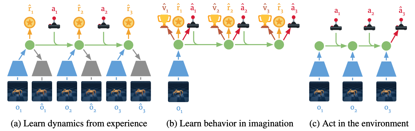
Latent World Model
- Encoder \(e_\phi(\mathbf{o}_t)\) compresses raw observation \(\mathbf{o}_t\) into a latent state \(\mathbf{z}_t\).
- Recurrent Transition \(p_\theta(\mathbf{z}_{t+1}\mid \mathbf{z}_t, a_t)\) predicts the next latent, plus a reward model \(\hat{r}_\theta(\mathbf{z}_t,a_t)\).
- Decoder \(d_\phi(\mathbf{z}_t)\) (optional) can reconstruct \(\mathbf{o}_t\) for training, but not necessarily used at inference.
Policy Learning in Imagination
-
An actor \(\pi_\psi(a_t\mid \mathbf{z}_t)\) and critic \(V_\psi(\mathbf{z}_t)\) are learned by backprop through the latent rollouts:
\[ \max_{\psi} \;\; \mathbb{E}_{\substack{\mathbf{z}_0 \sim q(\mathbf{z}_0|\mathbf{o}_0) \\ a_t \sim \pi_\psi(\cdot|\mathbf{z}_t) \\ \mathbf{z}_{t+1} \sim p_\theta(\cdot|\mathbf{z}_t,a_t)}}\!\biggl[\sum_{t=0}^{H-1} \gamma^t \hat{r}_\theta(\mathbf{z}_t, a_t)\biggr]. \] -
Dreamer uses advanced techniques (e.g., reparameterization, actor-critic with value expansion, etc.) to stabilize training.
Highlights
- DreamerV1: SOTA results on DM Control from image inputs.
- DreamerV2: Extended to Atari, surpassing DQN with a single architecture.
- DreamerV3: Achieved multi-domain generality (Atari, ProcGen, DM Control, robotics, Minecraft). The first algorithm to solve “collect a diamond” in Minecraft from scratch without demonstrations.
Significance
- Demonstrates that purely learning a latent world model + training by imagination can match or surpass leading model-free methods in terms of both sample efficiency and final returns.
7.5 MuZero (DeepMind, 2020)
Core Idea
Combines Monte Carlo Tree Search (MCTS) with a learned latent state to achieve superhuman performance on Go, Chess, Shogi, and set records on Atari—without knowing the environment’s rules explicitly.
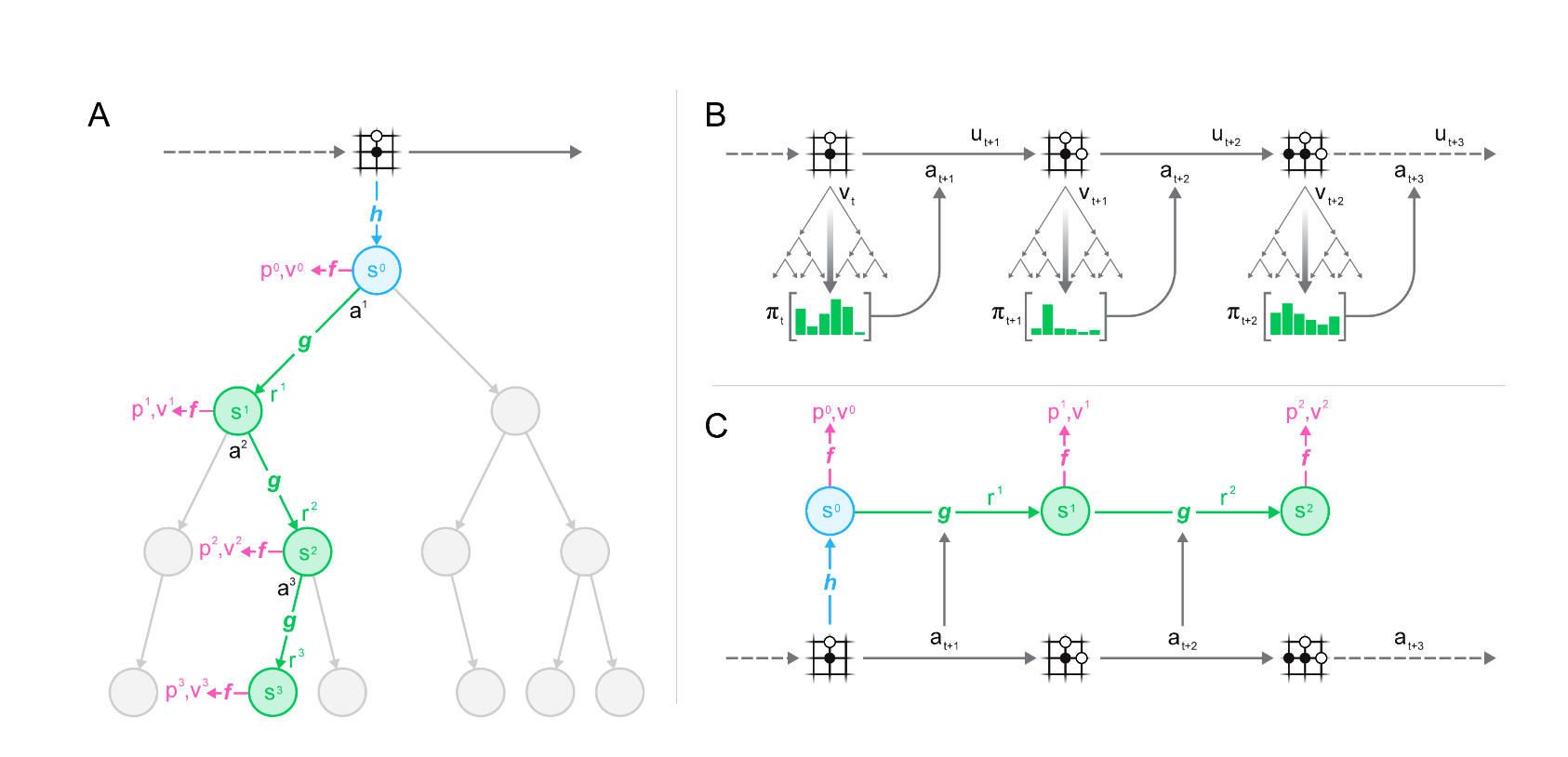
Network Architecture
- Representation Function \(h\):
- Maps the observation history to a latent state \(s_0 = h(\mathbf{o}_{1:t})\).
- Dynamics Function \(g\):
- Predicts the next latent state \(s_{k+1}=g(s_k, a_k)\) and immediate reward \(r_k\).
- Prediction Function \(f\):
- From a latent state \(s_k\), outputs a policy \(\pi_k\) (action logits) and a value \(v_k\).
MCTS in Latent Space
- Starting from \(s_0\), expand a search tree by simulating actions via \(g\).
- Each node stores mean value estimates \(\hat{V}\), visit counts, etc.
- The final search policy \(\alpha\) is used to update the network (target policy), and the environment reward is used to refine the reward/dynamics parameters.
Key Equations
-
MuZero is trained to minimize errors in reward, value, and policy predictions:
\[ \mathcal{L}(\theta) = \sum_{t=1}^{T} \bigl(\ell_\mathrm{value}(v_\theta(s_t), z_t) + \ell_\mathrm{policy}(\pi_\theta(s_t), \pi_t) + \ell_\mathrm{dyn}\bigl(g_\theta(s_t, a_t), s_{t+1}\bigr)\bigr), \]
with \(\pi_t\) and \(z_t\) from the improved MCTS-based targets.
Achievements
- Matches AlphaZero performance on Go, Chess, Shogi, but without an explicit rules model.
- Set new records on Atari-57.
- Demonstrates that an end-to-end learned model can be as effective for MCTS as a known simulator, provided it is trained to be “value-equivalent” (predict future rewards and values accurately).
Impact
- Showed that “learning to model the environment’s reward and value structure is enough”—MuZero does not need pixel-perfect next-state reconstructions.
- Successfully extended MCTS-based planning to domains with unknown or complex dynamics.
8. Key Benefits (and Drawbacks) of MBRL
8.1 Data Efficiency
MBRL can yield higher sample efficiency:
- Simulating transitions in the model extracts more learning signal from each real step
- E.g., PETS, MBPO, Dreamer require fewer environment interactions than top model-free methods
8.2 Exploration
A learned uncertainty-aware model can direct exploration to uncertain states:
- Bayesian or ensemble-based MBRL
- Potentially more efficient than naive \(\epsilon\)-greedy in high dimensions
8.3 Optimality
With a perfect model, MBRL can find better or equal policies vs. model-free. But if the model is imperfect, compounding errors can lead to suboptimal solutions. Research aims to close that gap (MBPO, Dreamer, MuZero).
8.4 Transfer
A global dynamics model can be re-used across tasks or reward functions:
- E.g., a learned robotic physics model can quickly adapt to new goals
- Saves extensive retraining
8.5 Safety
In real-world tasks (robotics, healthcare), we can plan or verify constraints inside the model before acting. Uncertainty estimation is crucial.
8.6 Explainability
A learned model can sometimes be probed or visualized, offering partial interpretability (though deep generative models remain somewhat opaque).
8.7 Disbenefits
- Model bias: Imperfect models => compounding errors
- Computational overhead: Planning can be expensive
- Implementation complexity: We must keep models accurate, stable, and do policy updates in tandem
9. Conclusion
Model-Based RL integrates planning and learning in the RL framework, offering strong sample efficiency and structured decision-making. Algorithms like MBPO, Dreamer, and MuZero demonstrate that short rollouts, uncertainty estimates, or latent value-equivalent models can yield high final performance with fewer real samples.
Still, challenges remain:
- Robustness under partial observability, stochastic transitions, or non-stationary tasks
- Balancing planning vs. data collection adaptively
- Scaling to high-dimensional, real-world tasks with safety constraints
Future work includes deeper hierarchical methods, advanced uncertainty modeling, bridging theory and practice, and constructing more interpretable or structured models.
10. References
-
S. Levine (CS 294-112: Deep RL)
Model-Based Reinforcement Learning, Lecture 9 slides.
Lecture Site, Video Repository
Additional resources: Open course materials from UC Berkeley’s Deep RL class -
T. Moerland et al. (2022)
“Model-based Reinforcement Learning: A Survey.” arXiv:2006.16712v4
Additional resources: Official GitHub for references and code snippets mentioned in the paper -
Sutton, R.S. & Barto, A.G.
Reinforcement Learning: An Introduction (2nd edition). MIT Press, 2018.
Online Draft
Additional resources: Exercise solutions and discussion forum -
Puterman, M.L.
Markov Decision Processes: Discrete Stochastic Dynamic Programming. John Wiley & Sons, 2014.
Publisher Link
Additional resources: Various lecture slides summarizing MDP fundamentals -
Deisenroth, M. & Rasmussen, C.E. (2011)
PILCO: A Model-Based and Data-Efficient Approach to Policy Search. ICML.
Paper PDF
Additional resources: Official code release on GitHub -
Chua, K. et al. (2018)
“Deep Reinforcement Learning in a Handful of Trials using Probabilistic Dynamics Models (PETS).” NeurIPS.
Paper Link
Additional resources: Author’s implementation -
Janner, M. et al. (2019)
“When to Trust Your Model: Model-Based Policy Optimization.” NeurIPS (MBPO).
Paper Link
Additional resources: Berkeley AI Research blog post -
Hafner, D. et al. (2020–2023)
“Dreamer” line of papers (ICML, arXiv).
DreamerV2 Code, Dreamer Blog
Additional resources: Tutorial videos by Danijar Hafner on latent world models -
Ha, D. & Schmidhuber, J. (2018)
“World Models.” NeurIPS.
Paper PDF, Project Site
Additional resources: Interactive demos and blog articles from David Ha -
Silver, D. et al. (various)
AlphaGo, AlphaZero, MuZero lines of research.
DeepMind’s MuZero Blog
Additional resources: Further reading on MCTS, AlphaGo, and AlphaZero in “Mastering the Game of Go” series