Week 4: Advanced Methods

Screen Record

Recitation Notes

Actor_Critic

The variance of policymethods can originate from two sources:

high variance in the cumulative reward estimate and
high variance in the gradient estimate.

For both problems, a solution has been developed: bootstrapping for better reward estimates and baseline subtraction to lower the variance of gradient estimates.

In the next seciton we will review the concepts bootstrapping (reward to go), using baseline (Advantage value) and Generalized Advantage Estimation (GAE).

Reward to Go:

A cumulative reward from state \(s_t\) to the end of the episode by applying policy \(\pi_\theta\).

As mentioned earlier, in the policy gradient method, we update our policy weights with the learning rate \(\alpha\) as follows:

\[ \theta \leftarrow \theta + \alpha \nabla_\theta J(\theta), \]

where

\[ \nabla_\theta J(\theta) \approx \frac{1}{N} \sum^N_{i=1} \sum^T_{t=1} \nabla_\theta \log\pi_\theta(a_{i,t}|s_{i,t})\cdot r(s_{i,t},a_{i,t}). \]

In this equation, the term \(r(s_{i,t}, a_{i,t})\) is the primary source of variance and noise. We use the causality trick to mitigate this issue by multiplying the policy gradient at state \(s_t\) with its future rewards. It is important to note that the policy at state \(s_t\) can only affect future rewards, not past ones. The causality trick is represented as follows:

\[ \nabla_\theta J(\theta) \approx \frac{1}{N} \sum^N_{i=1}\bigg( \sum^T_{t=1} \nabla_\theta \log\pi_\theta(a_{i,t}|s_{i,t})\bigg) \bigg( \sum^T_{t=1}r(s_{i,t},a_{i,t}) \bigg) \approx \frac{1}{N} \sum^N_{i=1} \sum^T_{t=1} \nabla_\theta \log\pi_\theta(a_{i,t}|s_{i,t})\bigg( \sum^T_{t'=t}r(s_{i,t'},a_{i,t'}) \bigg). \]

The term \(\sum^T_{t'=t}r(s_{i,t'},a_{i,t'})\) is known as reward to go, which is calculated in a Monte Carlo manner. It represents the total expected reward from a given state by applying policy \(\pi_\theta\), starting from time \(t\) to the end of the episode.

To further reduce variance, we can approximate the reward to go with the Q-value, which conveys a similar meaning. Thus, we can rewrite \(\nabla_\theta J(\theta)\) as:

\[ \nabla_\theta J(\theta) \approx \frac{1}{N} \sum^N_{i=1} \sum^T_{t=1} \nabla_\theta \log\pi_\theta(a_{i,t}|s_{i,t}) Q(s_{i,t},a_{i,t}). \]

Advantage Value:

Measures how much an action is better than the average of other actions in a given state.

Why Use the Advantage Value?

We can further reduce variance by subtracting a baseline from \(Q(s_{i,t}, a_{i,t})\) without altering the expectation of \(\nabla_\theta J(\theta)\), making it an unbiased estimator:

\[ \nabla_\theta J(\theta) \approx \frac{1}{N} \sum^N_{i=1} \sum^T_{t=1} \nabla_\theta \log\pi_\theta(a_{i,t}|s_{i,t}) \bigg( Q(s_{i,t},a_{i,t}) - b_t \bigg). \]

A reasonable choice for the baseline is the expected reward. Although it is not optimal, it significantly reduces variance.

We define:

\[ Q(s_{i,t},a_{i,t}) = \sum_{t'=t}^T E_{\pi_\theta}[r(s_{t'}, a_{t'})|s_t,a_t]. \]

To ensure the baseline is independent of the action taken, we compute the expectation of \(Q(s_{i,t}, a_{i,t})\) over all actions sampled from the policy:

\[ E_{a_t \sim \pi_\theta(a_{i,t}|s_{i,t})} [Q(s_{i,t},a_{i,t})] = V(s_t) = b_t. \]

Thus, the variance-reduced policy gradient equation becomes:

\[ \nabla_\theta J(\theta) \approx \frac{1}{N} \sum^N_{i=1} \sum^T_{t=1} \nabla_\theta \log\pi_\theta(a_{i,t}|s_{i,t}) \bigg( Q(s_{i,t},a_{i,t}) - V(s_t) \bigg). \]

We define the advantage function as:

\[ A(s_t,a_t) = Q(s_{i,t},a_{i,t}) - V(s_t). \]

Understanding the Advantage Function

Consider a penalty shootout game to illustrate the concept of the advantage function and Q-values in reinforcement learning.

# Game Setup:

A goalie always jumps to the right to block the shot.
A kicker can shoot either left or right with equal probability (0.5 each), defining the kicker's policy \(\pi_k\).

The reward matrix for the game is:

Kicker / Goalie	Right (jumps right)	Left (jumps left)
Right (shoots right)	0,1	1,0
Left (shoots left)	1,0	0,1

# Expected Reward:

Since the kicker selects left and right with equal probability, the expected reward is:

\[ V^{\pi_k}(s_t) = 0.5 \times 1 + 0.5 \times 0 = 0.5. \]

# Q-Value Calculation:

The Q-value is expressed as:

\[ Q^{\pi_k}(s_{i,t},a_{i,t}) = V^{\pi_k}(s_t) + A^{\pi_k}(s_t,a_t). \]

If the kicker shoots right, the shot is always saved (\(Q^{\pi_k}(s_{i,t},r) = 0\)).
If the kicker shoots left, the shot is always successful (\(Q^{\pi_k}(s_{i,t},l) = 1\)).

# Advantage Calculation:

The advantage function \(A^{\pi_k}(s_t,a_t)\) measures how much better or worse an action is compared to the expected reward.

If the kicker shoots left, he scores (reward = 1), which is 0.5 more than the expected reward \(V^{\pi_k}(s_t)\). Thus, the advantage of shooting left is:

\[ 1 = 0.5 + A^{\pi_k}(s_t,l) \Rightarrow A^{\pi_k}(s_t,l) = 0.5. \]

If the kicker shoots right, he fails (reward = 0), which is 0.5 less than the expected reward. Thus, the advantage of shooting right is:

\[ 0 = 0.5 + A^{\pi_k}(s_t,r) \Rightarrow A^{\pi_k}(s_t,r) = -0.5. \]

Estimating the Advantage Value

Instead of maintaining separate networks for estimating \(V(s_t)\) and \(Q(s_{i,t}, a_{i,t})\), we approximate \(Q(s_{i,t}, a_{i,t})\) using \(V(s_t)\):

\[ Q(s_{i,t},a_{i,t}) = r(s_t, a_t) + \sum_{t'=t+1}^T E_{\pi_\theta}[r(s_{t'}, a_{t'})|s_t,a_t] \approx r(s_t, a_t) + V(s_{t+1}). \]

Thus, we estimate the advantage function as:

\[ A(s_{i,t},a_{i,t}) \approx r(s_t, a_t) + V(s_{t+1}) - V(s_t). \]

We can also, consider the advantage function with discount factor as:

\[ A(s_{i,t},a_{i,t}) \approx r(s_t, a_t) + \gamma V(s_{t+1}) - V(s_t). \]

To train the value estimator, we use Monte Carlo estimation.

Generalized Advantage Estimation (GAE)

To have a good balance between variance and bias, we can use the concept of GAE, which is firstly introduced in High-Dimensional Continuous Control Using Generalized Advantage Estimation.

At the first, we define \(\hat{A}^{(k)}(s_{i,t},a_{i,t})\) to understand this the GAE concept.

\[ \hat{A}^{(k)}(s_{i,t},a_{i,t}) = r(s_t, a_t) + \dots + \gamma^{k-1}r(s_{t+k-1}, a_{t+k-1}) + \gamma^k V(s_{t+k})- V(s_t). \]

So, we can write the \(\hat{A}^{(k)}(s_{i,t},a_{i,t})\) for \(k \in \{1, \infty\}\) as:

\[ \hat{A}^{(1)}(s_{i,t},a_{i,t}) = r(s_t, a_t) + \gamma V(s_{t+1}) - V(s_t) \]

\[ \hat{A}^{(2)}(s_{i,t},a_{i,t}) = r(s_t, a_t) + \gamma r(s_{t+1}, a_{t+1}) + \gamma^2 V(s_{t+2}) - V(s_t) \]

\[ .\\ .\\ .\\ \]

\[ \hat{A}^{(\infty)}(s_{i,t},a_{i,t}) = r(s_t, a_t) + \gamma r(s_{t+1}, a_{t+1}) + \gamma^2 r(s_{t+2}, a_{t+2})+ \dots - V(s_t)\\ \]

\(\hat{A}^{(1)}(s_{i,t},a_{i,t})\) is high bias, low variance, whilst \(\hat{A}^{(\infty)}(s_{i,t},a_{i,t})\) is unbiased, high variance.

We take a weighted average of all \(\hat{A}^{(k)}(s_{i,t},a_{i,t})\) for \(k \in \{1, \infty\}\) with weight \(w_k = \lambda^{k-1}\) to balance bias and variance. This is called Generalized Advantage Estimation (GAE).

\[ \hat{A}^{(GAE)}(s_{i,t},a_{i,t}) = \frac{\sum_{k =1}^T w_k \hat{A}^{(k)}(s_{i,t},a_{i,t})}{\sum_k w_k}= \frac{\sum_{k =1}^T \lambda^{k-1} \hat{A}^{(k)}(s_{i,t},a_{i,t})}{\sum_k w_k} \]

Actor_Critic Algorihtms

Batch actor-critic algorithm

The first algorithm is: Actor-Critic with Bootstrapping and Baseline Subtraction In this algorithm, the simulator runs for an entire episode before updating the policy.

Batch actor-critic algorithm:

for each episode do:
for each step do:
Take action \(a_t \sim \pi_{\theta}(a_t | s_t)\), get \((s_t,a_t,s'_t,r_t)\).
Fit \(\hat{V}(s_t)\) with sampled rewards.
Evaluate the advantage function: \(A({s_t, a_t})\)
Compute the policy gradient: \(\nabla_{\theta} J(\theta) \approx \sum_{i} \nabla_{\theta} \log \pi_{\theta}(a_i | s_i) A({s_t})\)
Update the policy parameters: \(\theta \gets \theta + \alpha \nabla_{\theta} J(\theta)\)

Running full episodes for a single update is inefficient as it requires a significant amount of time. To address this issue, the online actor-critic algorithm is proposed.

Online actor-critic algorithm

In this algorithm, we take an action in the environment and immediately apply an update using that action.

Online actor-critic algorithm

for each episode do:
for each step do:
Take action \(a_t \sim \pi_{\theta}(a_t | s_t)\), get \((s_t,a_t,s'_t,r_t)\).
Fit \(\hat{V}(s_t)\) with the sampled reward.
Evaluate the advantage function: \(A({s,a})\)
Compute the policy gradient: \(\nabla_{\theta} J(\theta) \approx \nabla_{\theta} \log \pi_{\theta}(a | s) A({s,a})\)
Update the policy parameters: \(\theta \gets \theta + \alpha \nabla_{\theta} J(\theta)\)

Training neural networks with a batch size of 1 leads to high variance, making the training process unstable.

To mitigate this issue, two main solutions are commonly used: 1. Parallel Actor-Critic (Online) 2. Off-Policy Actor-Critic

Parallel Actor-Critic (Online)

Many high-performance implementations are based on the actor critic approach. For large problems, the algorithm is typically parallelized and implemented on a large cluster computer.

To reduce variance, multiple actors are used to update the policy. There are two main approaches:

Synchronized Parallel Actor-Critic: All actors run synchronously, and updates are applied simultaneously. However, this introduces synchronization overhead, making it impractical in many cases.
Asynchronous Parallel Actor-Critic: Each actor applies its updates independently, reducing synchronization constraints and improving computational efficiency. It also, uses asynchronous (parallel and distributed) gradient descent for optimization of deep neural network controllers.

Off-Policy Actor-Critic Algorithm

In the off-policy approach, we maintain a replay buffer to store past experiences, allowing us to train the model using previously collected data rather than relying solely on the most recent experience.

Off-policy actor-critic algorithm:

for each episode do:
for multiple steps do:
Take action \(a \sim \pi_{\theta}(a | s)\), get \((s,a,s',r)\), store in \(\mathcal{R}\).
Sample a batch \(\{s_i, a_i, r_i, s'_i \}\) for buffer \(\mathcal{R}\).
Fit \(\hat{Q}^{\pi}(s_i, a_i)\) for each \(s_i, a_i\).
Compute the policy gradient: \(\nabla_{\theta} J(\theta) \approx \frac{1}{N} \sum_{i} \nabla_{\theta} \log \pi_{\theta}(a^{\pi}_i | s_i) \hat{Q}^{\pi}(s_i, a^{\pi}_i)\)
Update the policy parameters: \(\theta \gets \theta + \alpha \nabla_{\theta} J(\theta)\)

To work with off-policy methods, we use the Q-value instead of the V-value in step 3. In step 4, rather than using the advantage function, we directly use \(\hat{Q}^{\pi}(s_i, a^{\pi}_i)\), where \(a^{\pi}_i\) is sampled from the policy \(\pi\). By using the Q-value instead of the advantage function, we do not encounter the high-variance problem typically associated with single-step updates. This is because we sample a batch from the replay buffer, which inherently reduces variance. As a result, there is no need to compute an explicit advantage function for variance reduction.

Issues with Standard Policy Gradient Methods

Earlier policy gradient methods, such as Vanilla Policy Gradient (VPG) or REINFORCE, suffer from high variance and instability in training. A key problem is that large updates to the policy can lead to drastic performance degradation.

To address these issues, Trust Region Policy Optimization (TRPO) was introduced, enforcing a constraint on how much the policy can change in a single update. However, TRPO is computationally expensive because it requires solving a constrained optimization problem. PPO is a simpler and more efficient alternative to TRPO, designed to ensure stable policy updates without requiring complex constraints.

Proximal Policy Optimization (PPO)

The intuition behind PPO

The idea with Proximal Policy Optimization (PPO) is that we want to improve the training stability of the policy by limiting the change you make to the policy at each training epoch: we want to avoid having too large policy updates. why?

We know empirically that smaller policy updates during training are more likely to converge to an optimal solution.
If we change the policy too much, we may end up with a bad policy that cannot be improved.

soruce: Unit 8, of the Deep Reinforcement Learning Class with Hugging Face

Therefore, in order not to allow the current policy to change much compared to the previous policy, we limit the ratio of these two policies to \([1 - \epsilon, 1 + \epsilon]\).

the Clipped Surrogate Objective

\[ L^{CLIP}(\theta) = \hat{\mathbb{E}}_t \left[ \min \left( r_t(\theta) \hat{A}_t, \text{clip} \left( r_t(\theta), 1 - \epsilon, 1 + \epsilon \right) \hat{A}_t \right) \right] \]

The ratio Function

\[ r_t(\theta) = \frac{\pi_{\theta}(a_t | s_t)}{\pi_{\theta_{\text{old}}}(a_t | s_t)} \]

\(r_{\theta}\) denotes the probability ratio between the current and old policy. if \(r_{\theta} > 1\), then the probability of doing action \(a_t\) at \(s_t\) in current policy is higher than the old policy and vice versa.

So this probability ratio is an easy way to estimate the divergence between old and current policy.

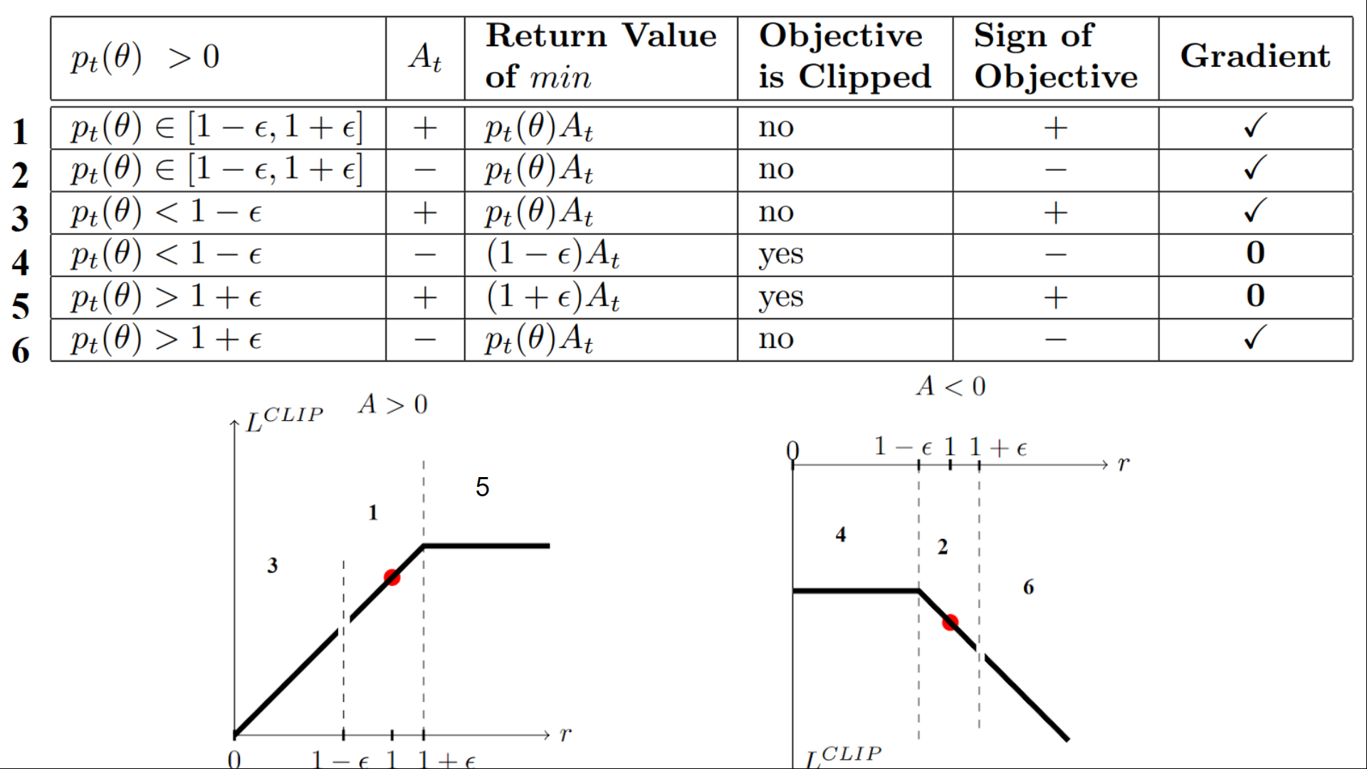
The clipped part

\[ \text{clip} \left( r_t(\theta), 1 - \epsilon, 1 + \epsilon \right) \hat{A}_t \]

If the current policy is updated significantly, such that the new policy parameters \(\theta'\) diverge greatly from the previous ones, the probability ratio between the new and old policies is clipped to the bounds \(1 - \epsilon\), \(1 + \epsilon\). At this point, the derivative of the objective function becomes zero, effectively preventing further updates.

The unclipped part

\[ r_t(\theta) \hat{A}_t \]

In the context of optimization, if the initial starting point is not ideal—i.e., if the probability ratio between the new and old policies is outside the range of \(1 - \epsilon\) and \(1 + \epsilon\)—the ratio is clipped to these bounds. This clipping results in the derivative of the objective function becoming zero, meaning no gradient is available for updates.

In this formulation, the optimization is performed with respect to the new policy parameters \(\theta'\), and \(A\) represents the advantage function, which indicates how much better or worse the action performed is compared to the average return.

Case 1: Positive Advantage (\(A > 0\))

if the Advantage \(A\) is positive (indicating that the action taken has a higher return than the expected return), and \(\frac{\pi_{\theta}(a_t | s_t)}{\pi_{\theta_{\text{old}}}(a_t | s_t)} < 1-\epsilon\) , the unclipped part is less than the clipped part and then it is minimized, so we have gradient to update the policy. This allows the policy to increase the probability of the action, aiming for the ratio to reach \(1 + \epsilon\) without violating the clipping constraint.

Case 2: Negative Advantage (\(A < 0\))

On the other hand, if the Advantage \(A\) is negative (meaning the action taken is worse than the average return), and \(\frac{\pi_{\theta}(a_t | s_t)}{\pi_{\theta_{\text{old}}}(a_t | s_t)} > 1+\epsilon\), the unclipped objective is again minimized and the gradient is non-zero, leading to an update. In this case, since the Advantage is negative, the policy is adjusted to reduce the probability of selecting that action, bringing the ratio closer to the boundary (\(1-\epsilon\)), while ensuring that the new policy does not deviate too much from the old one.

Visualize the Clipped Surrogate Objective

PPO pseudocode

Algorithm 1: PPO-Clip

Input: initial policy parameters \(\theta_0\), initial value function parameters \(\phi_0\)
for \(k = 0, 1, 2, \dots\) do
Collect set of trajectories \(\mathcal{D}_k = \{\tau_i\}\) by running policy \(\pi_k = \pi(\theta_k)\) in the environment.
Compute rewards-to-go \(\hat{R}_t\).
Compute advantage estimates, \(\hat{A}_t\) (using any method of advantage estimation) based on the current value function \(V_{\phi_k}\).
Update the policy by maximizing the PPO-Clip objective:

\[ \theta_{k+1} = \arg \max_{\theta} \frac{1}{|\mathcal{D}_k| T} \sum_{\tau \in \mathcal{D}_k} \sum_{t=0}^{T} \min \left( \frac{\pi_{\theta}(a_t | s_t)}{\pi_{\theta_k}(a_t | s_t)} A^{\pi_{\theta_k}}(s_t, a_t), \, g(\epsilon, A^{\pi_{\theta_k}}(s_t, a_t)) \right) \]

typically via stochastic gradient ascent with Adam.
Fit value function by regression on mean-squared error:

\[ \phi_{k+1} = \arg \min_{\phi} \frac{1}{|\mathcal{D}_k| T} \sum_{\tau \in \mathcal{D}_k} \sum_{t=0}^{T} \left( V_{\phi}(s_t) - \hat{R}_t \right)^2 \]
end for

Challenges of PPO algorithm

PPO requires a significant amount of interactions with the environment to converge. This can be problematic in real-world applications where data is expensive or difficult to collect. in fact it is a sample inefficient algorithm.

Hyperparameter Sensitivity: PPO requires careful tuning of hyperparameters such as the clipping parameter (epsilon), learning rate, and the number of updates per iteration. Poorly chosen hyperparameters can lead to suboptimal performance or even failure to converge.
Sample Efficiency: Although PPO is more sample-efficient than some other policy gradient methods, it still requires a significant amount of data to achieve good performance. This can be problematic in environments where data collection is expensive or time-consuming.
Exploration-Exploitation Tradeoff: PPO, like other policy gradient methods, can struggle with balancing exploration and exploitation. It may prematurely converge to suboptimal policies if it fails to explore sufficiently.

Helpful links

Unit 8, of the Deep Reinforcement Learning Class with Hugging Face

Proximal Policy Optimization (PPO) Explained

Proximal Policy Optimization (PPO) - How to train Large Language Models

Proximal Policy Optimization

Understanding PPO: A Game-Changer in AI Decision-Making Explained for RL Newcomers

Proximal Policy Optimization (PPO) - Explained

Deep Deterministic Policy Gradients (DDPG)

Handling Continuous Action Spaces

Why is this a problem?

In discrete action spaces, methods like DQN (Deep Q-Networks) can use an action-value function \(Q(s, a)\) to select the best action. However, in continuous action spaces, selecting the optimal action requires solving a high-dimensional optimization problem at every step, which is computationally expensive.

How does DDPG solve it?

DDPG uses a deterministic policy network \(\pi(s)\), which directly maps states to actions, eliminating the need for iterative optimization over action values.

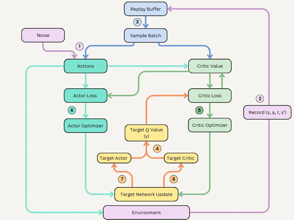
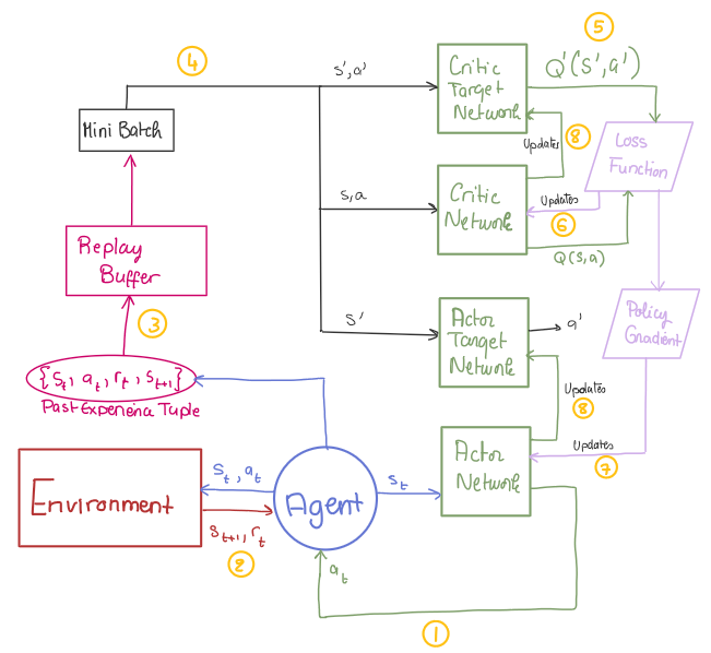
DDPG Architecture

DDPG uses four neural networks:
- A Q network
- A deterministic policy network
- A target Q network
- A target policy network

The Q network and policy network are similar to Advantage Actor-Critic (A2C), but in DDPG, the Actor directly maps states to actions (the output of the network directly represents the action) instead of outputting a probability distribution over a discrete action space.

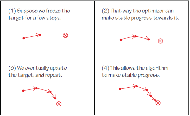
The target networks are time-delayed copies of their original networks that slowly track the learned networks. Using these target value networks greatly improves stability in learning.

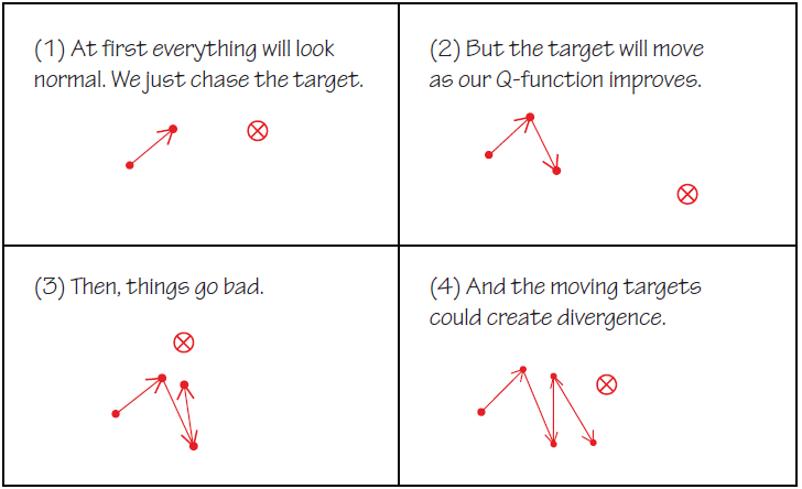
Why Use Target Networks?

In methods without target networks, the update equations of the network depend on the network's own calculated values, making it prone to divergence.

For example, if we update the Q-values directly using the current network, errors can compound, leading to instability. The target networks help mitigate this issue by providing more stable targets for updates.

\[ Q(s_t, a_t) \leftarrow r_t + \gamma Q(s_{t+1}, \arg\max_{a'} Q(s_{t+1}, a')) \]

Breakdown of DDPG Components

Experience Replay
Actor & Critic Network Updates
Target Network Updates
Exploration

Replay Buffer

As used in Deep Q-Learning and other RL algorithms, DDPG also utilizes a replay buffer to store experience tuples:

\[ (state, action, reward, next\_state) \]

These tuples are stored in a finite-sized cache (replay buffer). During training, random mini-batches are sampled from this buffer to update the value and policy networks.

Why Use Experience Replay?

In optimization tasks, we want data to be independently distributed. However, in an on-policy learning process, the collected data is highly correlated.

By storing experience in a replay buffer and sampling random mini-batches for training, we break correlations and improve learning stability.

Actor (Policy) & Critic (Value) Network Updates

Value Network (Critic) Update

The value network is updated similarly to Q-learning. The updated Q-value is obtained using the Bellman equation:

\[ y_i = r_i + \gamma Q' \left (s_{i+1}, \mu' (s_{i+1}|\theta^{\mu'})|\theta^{Q'} \right) \]

However, in DDPG, the next-state Q-values are calculated using the target Q network and target policy network.

Then, we minimize the mean squared error (MSE) loss between the updated Q-value and the original Q-value:

\[ \mathcal{L} = \frac{1}{N} \sum_{i} \left(y_i -Q(s_i, a_i|\theta^Q) \right)^2 \]

Note: The original Q-value is calculated using the learned Q-network, not the target Q-network.

Policy Network (Actor) Update

The policy function aims to maximize the expected return:

\[ J(\theta) = \mathbb{E} \left[ Q(s, a) \mid s = s_t, a_t = \mu(s_t) \right] \]

The policy loss is computed by differentiating the objective function with respect to the policy parameters:

\[ \nabla_{\theta^\mu} J(\theta) = \nabla_a Q(s, a) |_{a = \mu(s)} \nabla_{\theta^\mu} \mu(s|\theta^\mu) \]

But since we are updating the policy in an off-policy way with batches of experience, we take the mean of the sum of gradients calculated from the mini-batch:

\[ \nabla_{\theta_\mu} J(\theta) \approx \frac{1}{N} \sum_i \left[ \left. \nabla_a Q(s, a \mid \theta^Q) \right|_{s = s_i, a = \mu(s_i)} \nabla_{\theta_\mu} \mu(s \mid \theta^\mu) \Big|_{s = s_i} \right] \]

Target Network Updates

The target networks are updated via soft updates instead of direct copying:

\[ \theta^{Q'} \leftarrow \tau \theta^{Q} + (1 - \tau) \theta^{Q'} \]

\[ \theta^{\mu'} \leftarrow \tau \theta^{\mu} + (1 - \tau) \theta^{\mu'} \]

where \(\tau\) is a small value , ensuring smooth updates that prevent instability.

Exploration

In RL for discrete action spaces, exploration is often done using epsilon-greedy or Boltzmann exploration.

However, in continuous action spaces, exploration is done by adding noise to the action itself.

Ornstein-Uhlenbeck Process

The DDPG paper proposes adding Ornstein-Uhlenbeck (OU) noise to the actions.

The OU Process generates temporally correlated noise, preventing the noise from canceling out or "freezing" the action dynamics.

\[ \mu^{'}(s_t) = \mu(s_t|\theta^\mu_t) + \mathcal{N} \]

DDPG Pseudocode: A Step-by-Step Breakdown

Algorithm 1: DDPG Algorithm

Randomly initialize critic network \( Q(s, a | \theta^Q) \) and actor \( \mu(s | \theta^\mu) \) with weights \( \theta^Q \) and \( \theta^\mu \).
Initialize target networks \( Q' \) and \( \mu' \) with weights \( \theta^{Q'} \gets \theta^Q, \quad \theta^{\mu'} \gets \theta^\mu \).
Initialize replay buffer \( R \).

for episode = 1 to \( M \) do
  Initialize a random process \( \mathcal{N} \) for action exploration.
  Receive initial observation state \( s_1 \).
  for \( t = 1 \) to \( T \) do
    Select action \( a_t = \mu(s_t | \theta^\mu) + \mathcal{N}_t \) according to the current policy and exploration noise.
    Execute action \( a_t \) and observe reward \( r_t \) and new state \( s_{t+1} \).
    Store transition \( (s_t, a_t, r_t, s_{t+1}) \) in \( R \).
    Sample a random minibatch of \( N \) transitions \( (s_i, a_i, r_i, s_{i+1}) \) from \( R \).
    Set:

\[ y_i = r_i + \gamma Q'(s_{i+1}, \mu'(s_{i+1} | \theta^{\mu'}) | \theta^{Q'}) \]

Update critic by minimizing the loss:

\[ L = \frac{1}{N} \sum_i (y_i - Q(s_i, a_i | \theta^Q))^2 \]

Update actor policy using the sampled policy gradient:

\[ \nabla_{\theta^\mu} J \approx \frac{1}{N} \sum_i \nabla_a Q(s, a | \theta^Q) |_{s=s_i, a=\mu(s_i)} \nabla_{\theta^\mu} \mu(s | \theta^\mu) |_{s_i} \]

Update the target networks:

\[ \theta^{Q'} \gets \tau \theta^Q + (1 - \tau) \theta^{Q'} \]

\[ \theta^{\mu'} \gets \tau \theta^\mu + (1 - \tau) \theta^{\mu'} \]

end for
end for

Soft Actor-Critic (SAC)

Challenges and motivation of SAC

Previous Off-policy methods like DDPG often struggle with exploration , leading to suboptimal policies. SAC overcomes this by introducing entropy maximization, which encourages the agent to explore more efficiently.
Sample inefficiency is a major issue in on-policy algorithms like Proximal Policy Optimization (PPO), which require a large number of interactions with the environment. SAC, being an off-policy algorithm, reuses past experiences stored in a replay buffer, making it significantly more sample-efficient.
Another challenge is instability in learning, as methods like DDPG can suffer from overestimation of Q-values. SAC mitigates this by employing twin Q-functions (similar to TD3) and incorporating entropy regularization, leading to more stable and robust learning.

In essence, SAC seeks to maximize the entropy in policy, in addition to the expected reward from the environment. The entropy in policy can be interpreted as randomness in the policy.

what is entropy?

We can think of entropy as how unpredictable a random variable is. If a random variable always takes a single value then it has zero entropy because it’s not unpredictable at all. If a random variable can be any Real Number with equal probability then it has very high entropy as it is very unpredictable.

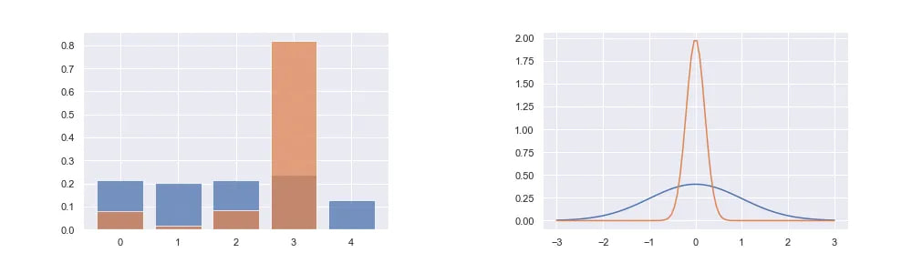
probability distributions with low entropy have a tendency to greedily sample certain values, as the probability mass is distributed relatively unevenly.

Maximum Entropy Reinforcement Learning

In Maximum Entropy RL, the agent tries to optimize the policy to choose the right action that can receive the highest sum of reward and long term sum of entropy. This enables the agent to explore more and avoid converging to local optima.

reason: We want a high entropy in our policy to encourage the policy to assign equal probabilities to actions that have same or nearly equal Q-values(allow the policy to capture multiple modes of good policies), and also to ensure that it does not collapse into repeatedly selecting a particular action that could exploit some inconsistency in the approximated Q function. Therefore, SAC overcomes the problem by encouraging the policy network to explore and not assign a very high probability to any one part of the range of actions.

The objective function of the Maximum entropy RL is as shown below:

\[ J(\pi_{\theta}) = \mathbb{E}_{\pi_{\theta}} \left[ \sum_{t=0}^{\infty} \gamma^t R(s_t, a_t) + \alpha H(\pi(\cdot | s_t)) \right] \]

and the optimal policy is:

\[ \pi^* = \arg\max_{\pi_{\theta}} \mathbb{E}_{\pi_{\theta}} \left[ \sum_{t=0}^{\infty} \gamma^t R(s_t, a_t) + \alpha H(\pi(\cdot | s_t)) \right] \]

\(\alpha\) is the temperature parameter that balances between exploration and exploitation.

Overcoming Exploration Bias in Multimodal Q-Functions

Here we want to explain the concept of a multimodal Q-function in reinforcement learning (RL), where the Q-value function, \(Q(s, a)\), represents the expected cumulative reward for taking action \(a\) in state \(s\).

In this context, the robot is in an initial state and has two possible passages to follow, which result in a bimodal Q-function (a function with two peaks). These peaks correspond to two different action choices, each leading to different potential outcomes.

Standard RL Approach

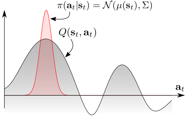
The grey curve represents the Q-function, which has two peaks, indicating two promising actions.A conventional RL approach typically assumes a unimodal (single-peaked) policy distribution, represented by the red curve.

This policy distribution is modeled as a Gaussian \(\mathcal{N}(\mu(s_t), \Sigma)\) centered around the highest Q-value peak.

This setup results in exploration bias where the agent primarily explores around the highest peak and ignores the lower peak entirely.

Improved Exploration Strategy

Instead of using a unimodal Gaussian policy, a Boltzmann-weighted policy is used. The policy distribution (green shaded area) is proportional to \(\exp(Q(s_t, a_t))\), meaning actions are sampled based on their Q-values.

This approach allows the agent to explore multiple high-reward actions and avoids the bias of ignoring one passage. As a result, the agent recognizes both options, increasing the chance of finding the optimal path.

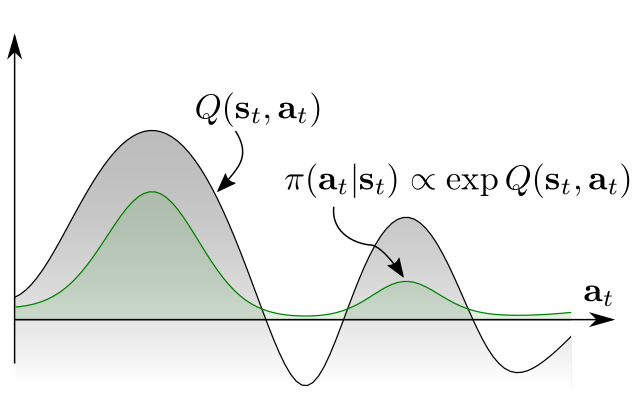
This concept is relevant for actor-critic RL methods like Soft Actor-Critic (SAC), which uses entropy to encourage diverse exploration.

Soft Policy

Soft policy

\[ J(\pi) = \sum_{t=0}^{T} \mathbb{E}_{(s_t, a_t)\sim\rho_{\pi}} \left[ r(s_t, a_t) + \alpha\mathcal{H}(\pi(\cdot | s_t)) \right] \]

With new objective function we need to define Value funciton and Q-value funciton again.

Soft Q-value funciton

\[ Q(s_t, a_t) = r(s_t, a_t) + \gamma\mathbb{E}_{s_{t+1}\sim p}\left[ V(s_{t+1}) \right] \]

Soft Value function

\[ V(s_t) = \mathbb{E}_{a_t\sim \pi} \left[Q(s_t, a_t) - \text{log}\space\pi(a_t|s_t)\right] \]

Soft policy iteration

Soft Policy Iteration is an entropy-regularized version of classical policy iteration, which consists of:

Soft Policy Evaluation: Estimating the soft Q-value function under the current policy.
Soft Policy Improvement: Updating the policy to maximize the soft Q-value function,incorporating entropy regularization.

This process iteratively improves the policy while balancing exploration and exploitation.

Soft Policy Evaluation (Critic Update)

The goal of soft policy evaluation is to compute the expected return of a given policy \(\pi\) under the maximum entropy objective, which modifies the standard Bellman equation by adding an entropy term. (SAC explicitly learns the Q-function for the current policy)

The soft Q-value function for a policy \(\pi\) is updated using a modified Bellman operator \(T^{\pi}\):

\[ T^\pi Q(s_t, a_t) = r(s_t, a_t) + \gamma \mathbb{E}_{s_{t+1} \sim p} [V(s_{t+1})] \]

with substitution of \(V\) we have :

\[ T^\pi Q(s_t, a_t) = r(s_t, a_t) + \gamma \mathbb{E}_{\substack{s_{t+1} \sim p \\ a_{t+1} \sim \pi}} [Q(s_{t+1,}, a_{t+1}) - \text{log}\space\pi(a_{t+1}|s_{t+1})] \]

Key Result: Soft Bellman Backup Convergence

Theorem: By repeatedly applying the operator \(T^\pi\), the Q-value function converges to the true soft Q-value function for policy \(\pi\):

\[ Q_k \to Q^\pi \text{ as } k \to \infty \]

Thus, we can estimate \(Q^\pi\) iteratively.

Soft Policy Improvement (Actor Update)

Once the Q-function is learned, we need to improve the policy using a gradient-based update. This means:

Instead of directly maximizing Q-values, the policy is updated to optimize a modified objective that balances reward maximization and exploration.
The update is off-policy, meaning the policy can be trained using past experiences stored in a replay buffer, rather than requiring fresh samples like on-policy methods (e.g., PPO).

The update is based on an exponential function of the Q-values:

\[ \pi^*(a | s) \propto \exp (Q^\pi(s, a)) \]

which means the optimal policy is obtained by normalizing \(\exp (Q^\pi(s, a))\) over all actions:

\[ \pi^*(a | s) = \frac{\exp (Q^\pi(s, a))}{Z^\pi(s)} \]

where \(Z^\pi(s)\) is the partition function that ensures the distribution sums to 1.

For the policy improvement step, we update the policy distribution towards the softmax distribution for the current Q function.

\[ \pi_{\text{new}} = \arg \min_{\pi' \in \Pi} D_{\text{KL}} \left( \pi'(\cdot | s) \, \bigg|\bigg| \, \frac{\exp (Q^\pi(s, \cdot))}{Z^\pi(s)} \right) \]

Key Result: Soft Policy Improvement Theorem
The new policy \(\pi_{\text{new}}\) obtained via this update improves the expected soft return:

\[ Q^{\pi_{\text{new}}}(s, a) \geq Q^{\pi_{\text{old}}}(s, a) \quad \forall (s, a) \]

Thus, iterating this process leads to a better policy.

Convergence of Soft Policy Iteration

By alternating between soft policy evaluation and soft policy improvement, soft policy iteration converges to an optimal maximum entropy policy within the policy class \(\Pi\):

\[ \pi^* = \arg \max_{\pi \in \Pi} \sum_t \mathbb{E}[r_t + \alpha H(\pi(\cdot | s_t))] \]

However, this exact method is only feasible in the tabular setting. For continuous control, we approximate it using function approximators.

Soft Actor-Critic

For complex learning domains with high-dimensional and/or continuous state-action spaces, it is mostly impossible to find exact solutions for the MDP. Thus, we must leverage function approximation (i.e. neural networks) to find a practical approximation to soft policy iteration. then we use stochastic gradient descent (SGD) to update parameters of these networks.

we model the value functions as expressive neural networks, and the policy as a Gaussian distribution over the action space with the mean and covariance given as neural network outputs with the current state as input.

Soft Value function (\(V_{\psi}(s)\))

A separate soft value function which helps in stabilising the training process. The soft value function approximator minimizes the squared residual error as follows:

\[ J_V(\psi) = \mathbb{E}_{s_{t} \sim \mathcal{D}} \left[ \frac{1}{2} \left( V_{\psi}(s_t) - \mathbb{E}_{a \sim \pi_{\phi}} [Q_{\theta}(s_t, a_t) - \log \pi_{\phi}(a_t | s_t)] \right)^2 \right] \]

It means the learning of the state-value function, \(V\) is done by minimizing the squared difference between the prediction of the value network and expected prediction of Q-function with the entropy of the policy, \(\pi\). - \(D\) is the distribution of previously sampled states and actions, or a replay buffer.

Gradient Update for \(V_{\psi}(s)\)

\[ \hat{\nabla}_{\psi} J_V(\psi) = \nabla_{\psi} V_{\psi}(s_t) \left( V_{\psi}(s_t) - Q_{\theta}(s_t, a_t) + \log \pi_{\phi}(a_t | s_t) \right) \]

where the actions are sampled according to the current policy, instead of the replay buffer.

Soft Q-funciton (\(Q_{\theta}(s, a)\))

We minimize the soft Q-function parameters by using the soft Bellman residual provided here:

\[ J_Q(\theta) = \mathbb{E}_{(s_{t}, a_t) \sim \mathcal{D}} \left[ \frac{1}{2} \left( Q_{\theta}(s_t, a_t) - \hat{Q}(s_t, a_t)\right)^2 \right] \]

with :

\[ \hat{Q}(s_t, a_t) = r(s_t, a_t) + \gamma \space \mathbb{E}_{s_{t+1} \sim p} [V_{\bar{\psi}}(s_{t+1})] \]

Gradient Update for \(Q_{\theta}\):

\[ \hat{\nabla}_\theta J_Q(\theta) = \nabla_{\theta} Q_{\theta}(s_t, a_t) \left( Q_{\theta}(s_t, a_t) - r(s_t, a_t) - \gamma V_{\bar{\psi}}(s_{t+1}) \right) \]

A target value function \(V_{\bar{\psi}}\) (exponentially moving average of \(V_{\psi}\)) is used to stabilize training.

More Explanation About Target Networks:

The use of target networks is motivated by a problem in training \(V\) network. If you go back to the objective functions in the Theory section, you will find that the target for the \(Q\) network training depends on the \(V\) Network and the target for the \(V\) Network depends on the \(Q\) network (this makes sense because we are trying to enforce Bellman Consistency between the two functions). Because of this, the \(V\) network has a target that’s indirectly dependent on itself which means that the \(V\) network’s target depends on the same parameters we are trying to train. This makes training very unstable.

The solution is to use a set of parameters which comes close to the parameters of the main \(V\) network, but with a time delay. Thus we create a second network which lags the main network called the target network. There are two ways to go about this.

The first way is to have the target network copied over from the main network regularly after a set number of steps -> Periodic Hard Update

\[ \theta^{-} \leftarrow \theta \]

The other way is to update the target network by Polyak averaging (a kind of moving averaging) itself and the main network. -> Soft Update

\[ \theta^{-} \leftarrow \tau \theta + (1-\tau) \theta^{-} \]

source: concept target network in category reinforcement learning

Policy network (\(\pi_{\phi}(a|s)\))

The policy \(\pi_{\phi}(a | s)\) is updated using the soft policy improvement step, minimizing the KL-divergence:

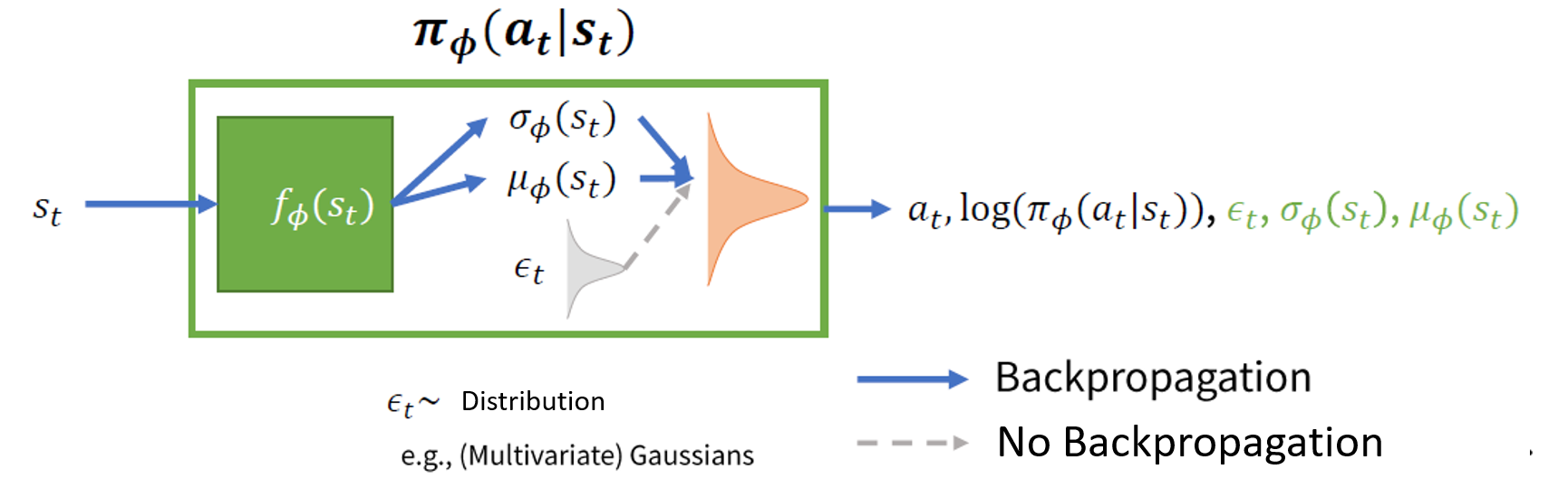
\[ J_{\pi}(\phi) = \mathbb{E}_{s_t \sim \mathcal{D}} \left[ D_{\text{KL}} \left( \pi_{\phi}(\cdot | s_t) \bigg\| \frac{\exp(Q_{\theta}(s_t, \cdot))}{Z_{\theta}(s_t)} \right) \right] \]

Instead of solving this directly, SAC reparameterizes the policy using:

\[ a_t = f_{\phi}(\epsilon_t; s_t) \]

This trick is used to make sure that sampling from the policy is a differentiable process so that there are no problems in backpropagating the errors. \(\epsilon_t\) is random noise vector sampled from fixed distribution (e.g., Spherical Gaussian).

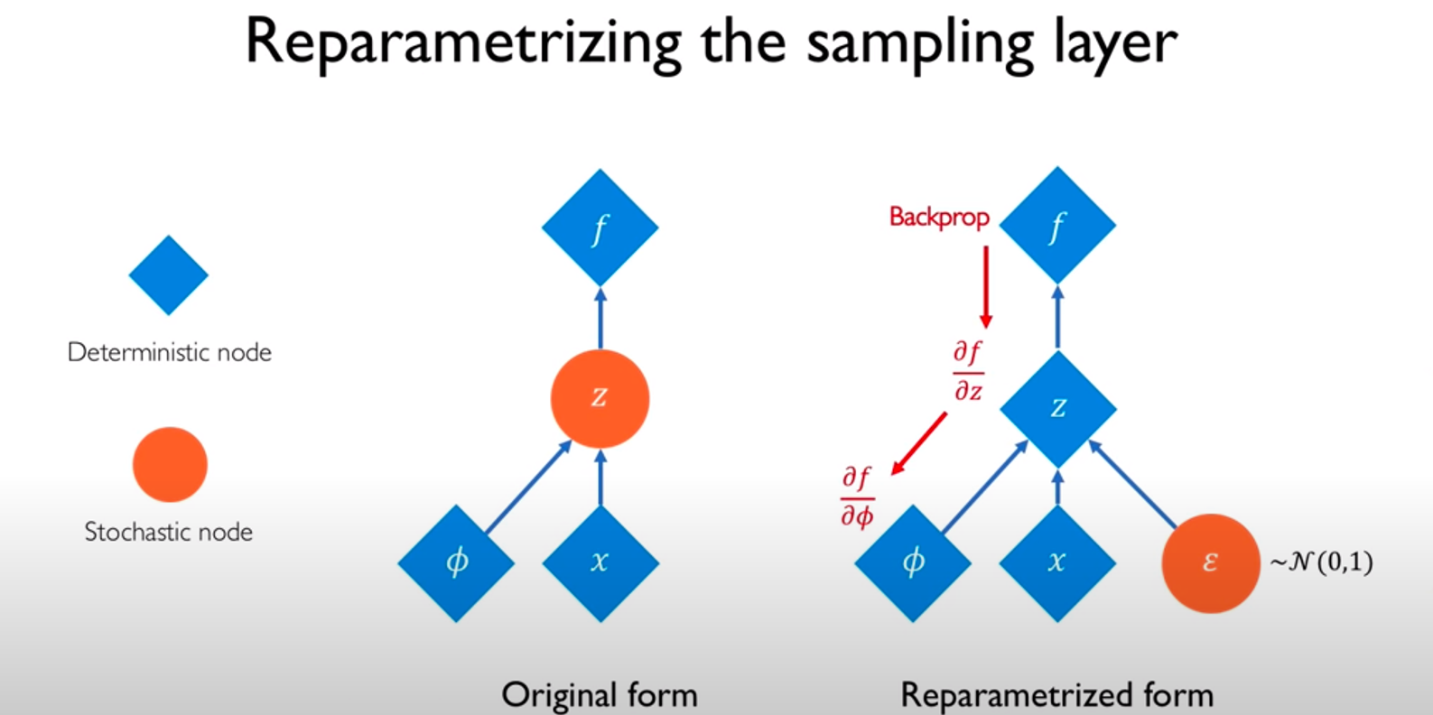
Why Reparameterization is Needed?

In reinforcement learning, the policy \(\pi(a | s)\) often outputs a probability distribution over actions rather than deterministic actions. The standard way to sample an action is:

\[ a_t \sim \pi_{\phi}(a_t | s_t) \]

However, this sampling operation blocks gradient flow during backpropagation, preventing efficient training using stochastic gradient descent (SGD).

Instead of directly sampling \(a_t\) from \(\pi_{\phi}(a_t | s_t)\), we transform a simple noise variable into an action:

\[ a_t = f_{\phi}(\epsilon_t, s_t) \]

\(\epsilon_t \sim \mathcal{N}(0, I)\) is sampled from a fixed noise distribution (e.g., a Gaussian).
\(f_{\phi}(\epsilon_t, s_t)\) is a differentiable function (often a neural network) that maps noise to an action.

For a Gaussian policy in SAC, the action is computed as:

\[ a_t = \mu_{\phi}(s_t) + \sigma_{\phi}(s_t) \cdot \epsilon_t \]

So instead of sampling from \(\mathcal{N}(\mu, \sigma^2)\) directly, we sample from a fixed standard normal and transform it using a differentiable function.This makes the policy differentiable, allowing gradients to flow through \(\mu_{\phi}\) and \(\sigma_{\phi}\).

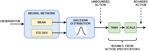
Continuous Action Generation

In a continuous action space soft actor-critic agent, the neural network in the actor takes the current observation and generates two outputs, one for the mean and the other for the standard deviation. To select an action, the actor randomly selects an unbounded action from this Gaussian distribution. If the soft actor-critic agent needs to generate bounded actions, the actor applies tanh and scaling operations to the action sampled from the Gaussian distribution.

During training, the agent uses the unbounded Gaussian distribution to calculate the entropy of the policy for the given observation.

Discrete Action Generation

In a discrete action space soft actor-critic agent, the actor takes the current observation and generates a categorical distribution, in which each possible action is associated with a probability. Since each action that belongs to the finite set is already assumed feasible, no bounding is needed.

During training, the agent uses the categorical distribution to calculate the entropy of the policy for the given observation.

if we rewrite the equation we have:

\[ J_{\pi}(\phi) = \mathbb{E}_{s_t \sim \mathcal{D}, \epsilon_t \sim \mathcal{N}} \left[ \text{log}\space\pi_{\phi} \left(f_{\phi}(\epsilon_t; s_t) | s_t \right) - Q_{\theta}(s_t,f_{\phi}(\epsilon_t; s_t) \right] \]

where \(\pi_{\phi}\) is defined implicitly in terms of \(f_{\phi}\), and we have noted that the partition function is independent of \(\phi\) and can thus be omitted.

Policy Gradient Update

\[ \hat{\nabla}_{\phi} J_{\pi}(\phi) = \nabla_{\phi} \log \pi_{\phi}(a_t | s_t) + \left( \nabla_{a_t} \log \pi_{\phi}(a_t | s_t)- \nabla_{a_t} Q_{\theta}(s_t, a_t) \right) \nabla_{\phi} f_{\phi}(\epsilon_t; s_t) \]

SAC pseudocode

Algorithm 1: Soft Actor-Critic

Initialize parameter vectors \(\psi, \bar{\psi}, \theta, \phi\)

for each iteration do
    for each environment step do
        \(a_t \sim \pi_{\phi}(a_t | s_t)\)
        \(s_{t+1} \sim p(s_{t+1} | s_t, a_t)\)
        \(\mathcal{D} \gets \mathcal{D} \cup \{(s_t, a_t, r(s_t, a_t), s_{t+1})\}\)
    end for

    for each gradient step do
        \(\psi \gets \psi - \lambda \hat{\nabla}_{\psi} J_V(\psi)\)
        \(\theta_i \gets \theta_i - \lambda_Q \hat{\nabla}_{\theta_i} J_Q(\theta_i) \quad \text{for } i \in \{1,2\}\)
        \(\phi \gets \phi - \lambda_{\pi} \hat{\nabla}_{\phi} J_{\pi}(\phi)\)
        \(\bar{\psi} \gets \tau \psi + (1 - \tau) \bar{\psi}\)
    end for
end for

Author(s)

Ahmad Karami

Teaching Assistant

ahmad.karami77@yahoo.com
Hamidreza Ebrahimpour

Teaching Assistant

ebrahimpour.7879@gmail.com