Week 6: Multi-Armed Bandits
Screen Record
Recitation Notes
1. Definition of the Problem
The multi-armed bandit problem is a very simple model that we can investigate to better understand the exploration/exploitation tradeoff. In this MDP, we have no state, but only actions and a reward function, i.e. \((\mathcal{A, R})\). Here, \(\mathcal{A}\) is a finite set of actions ("bandit arms"), while \(\mathcal{R}\) is a distribution over rewards for actions: \(\mathcal{R}^a(r) = \Pr[R = r | A = a]\). At each step, then, the agent selects an action \(A_t \in \mathcal{A}\) and the environment generates a reward ("payout") \(R_t \sim \mathcal{R}^{A_t}\). The goal, as always, is to maximize the cumulative reward \(\sum_{\tau=1}^t R_{\tau}\).
We can define a few more functions and variables in this setup. The action-value (Q-value) of an action is the mean reward for that action:
Furthermore, there exists one optimal value \(v_{\star}\), which is the Q-value of the best action \(a^{\star}\):
The difficulty lies in the fact that the agent does not initially know the reward distributions of the arms. It must balance exploration (gathering information about unknown arms) and exploitation (choosing the best-known arm) to optimize long-term gains.
Formally, the MAB problem consists of:
- A finite action set \(\mathcal{A}\) with \(k\) possible actions.
- A reward distribution \(\mathcal{R}^a\) for each action \(a\) where \(R_t \sim \mathcal{R}^{A_t}\) represents the reward obtained at time \(t\).
- The objective is to maximize the cumulative reward over \(T\) steps:
Non-Associativity Property
- Unlike full reinforcement learning problems, multi-armed bandits are non-associative.
- This means that the best action does not depend on the state; the optimal action is the same for all time steps.
- Formally, we do not consider state transitions: The bandit setting only involves selecting actions and receiving rewards, without any long-term effects from past decisions.
Unlike full Markov Decision Processes (MDPs), the MAB setting does not involve state transitions, meaning the agent must learn optimal actions purely through repeated trials.
Real-World Applications of MAB
The MAB framework is used in several fields:
- Medical Trials: Identifying the best treatment while minimizing patient risk.
- Online Advertising: Choosing optimal ad placements for revenue maximization.
- Recommendation Systems: Dynamically selecting personalized content.
- Financial Investments: Allocating assets to maximize returns under uncertainty.
2. Action-Value Methods and Types
To solve the MAB problem, we need a way to estimate action values. The action-value function \(Q_t(a)\) estimates the expected reward of choosing action \(a\) at time step \(t\):
We define sample-average estimation of \(Q_t(a)\) as:
where: - \(N_t(a)\) is the number of times action \(a\) has been selected. - \(R_i\) is the reward received when selecting \(a\).
Incremental Update Rule for Efficient Computation
Instead of storing all past rewards, we can update \(Q_t(a)\) incrementally:
Derivation
The sample-average estimate at time step \(t+1\) is:
Expanding this in terms of \(Q_t(a)\):
Since \(Q_t(a)\) is the average of previous rewards:
Multiplying by \(N_t(a)\):
Substituting into the equation:
Rewriting in update form:
This allows us to update \(Q_t(a)\) without storing all past rewards.
Constant Step-Size Update (For Nonstationary Problems)
When dealing with changing reward distributions, we use a constant step-size \(\alpha\):
where \(\alpha\) determines how much weight is given to recent rewards.
- If \(\alpha = \frac{1}{N_t(a)}\), this becomes sample-average estimation.
- If \(\alpha\) is constant, this results in exponentially weighted averaging, useful for nonstationary problems.
Exponential Weighted Averaging
Expanding recursively:
Expanding further:
This pattern continues, showing that older rewards have exponentially decaying influence:
which demonstrates the effect of exponential weighting.
3. Regret: Measuring Suboptimality
Furthermore, we'll now want to investigate a novel quantity known as the regret. Regret gives us an indication of the opportunity loss for picking a particular action \(A_t\) compared to the optimal action \(a^\star\) In symbols:
Finally, we can define the total regret as the total opportunity loss over an entire episode:
The goal of the agent is then to minimize the total regret, which is equivalent to maximizing the cumulative (total) reward. In addition to the above definitions, we'll now also keep a count \(N_t(a)\) which is the expected number of selections for an action a. Moreover, we define the gap \(\delta_a\) as the difference between the expected value \(q(a)\) of an action a and the optimal action:
As such, we can give an equivalent definition of the regret \(L_t\) in terms of the gap:
Now, if we think of the regret as a function of iterations, we can make some observations. For example, we observe that the regret of a greedy algorithm \(A_t = \text{argmax}_{a \in \mathcal{A}} Q_t(a)\) is a linear function, i.e. it increases linearly with each iteration. The reason why is that we may "lock" onto a suboptimal action forever, thus adding a certain fixed amount of regret each time. An alteration that we can make here is to initialize the Q-value of each action to the maximum reward. This is called optimistic initialization. Note that updates to \(Q(a)\) are made via an averaging process:
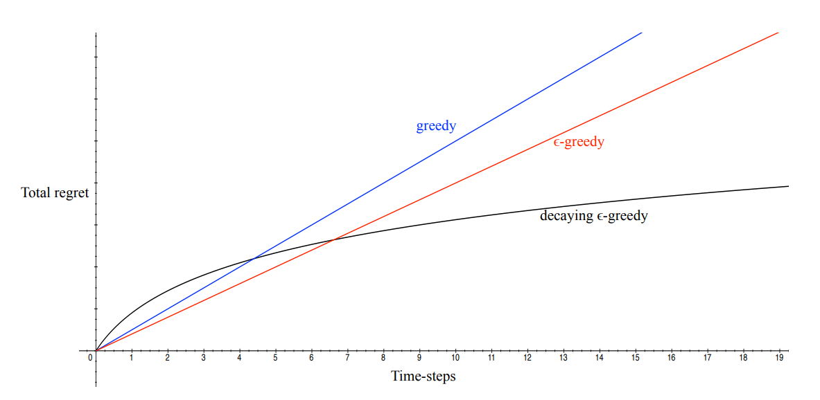
Now, while \(\varepsilon\)-greedy approaches incur linear regret, certain strategies that decay \(\varepsilon\) can actually only incur logarithmic (asymptotic) regret. Either way, there is actually a lower bound on the regret that any algorithm can achieve (i.e. no algorithm can do better), which is logarithmic:
As you can see, this lower bound is proportional to the gap size (higher gap size means higher lower-bound for regret, i.e. more regret) and indirectly proportional to the similarity of bandits, given by the Kullback-Leibler divergence.
4. Exploration-Exploitation Dilemma and Uncertainty
The exploration-exploitation tradeoff is at the heart of MAB problems:
- Exploitation: Selecting the action with the highest known reward.
- Exploration: Trying less-known actions to gather new information.
Since the agent lacks prior knowledge of the optimal action, exploration is necessary to reduce uncertainty. However, excessive exploration may lead to unnecessary loss of rewards. Finding the right balance is essential for optimal performance.
5. Exploration Strategies in Bandits
Several strategies help balance exploration and exploitation effectively:
5.1. \(\epsilon\)-Greedy Exploration
One of the simplest strategies for exploration is \(\epsilon\)-greedy, where:
- With probability \(1 - \epsilon\), we exploit by selecting the best-known action.
- With probability \(\epsilon\), we explore by selecting a random action.
A variation, decaying \(\varepsilon\)-greedy, reduces \(\varepsilon\) over time to favor exploitation as learning progresses.
5.2 Optimistic Initialization
Optimistic initialization encourages exploration by initializing action-values with an artificially high value:
This approach works by ensuring that initially, every action appears to be promising, forcing the agent to sample all actions before settling on an optimal choice. The key idea is to assume that each action is better than it actually is, prompting the agent to try them all.
In practice, an optimistic estimate is set as:
where \(R_{\max}\) is an upper bound on the highest possible reward. Since the agent updates estimates based on actual experience, actions with lower rewards will eventually have their values corrected downward, while the truly optimal actions will remain highly rated.
Optimistic initialization is particularly effective when: - The environment is stationary, meaning reward distributions do not change over time. - The number of actions is small, ensuring each action is explored adequately. - The upper bound estimate \(R_{\max}\) is not too high, as overly optimistic values can cause unnecessary exploration.
This method is simple yet effective for balancing exploration and exploitation, particularly when rewards are initially unknown. method ensures early exploration before settling on the best action.
5.3 UCB
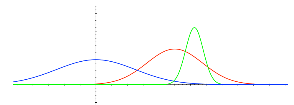
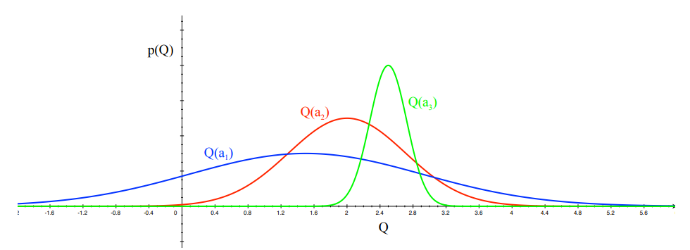
A very fundamental idea within the exploration/exploitation domain is that of optimism in the face of uncertainty. This idea tells us that if we know very well of the value of one action, but not as well about the value of another action, but do know that that other value may have a greater value, then we should go for the other action. So if you imagine a Gaussian distribution for the first action and a Gaussian for the second, then if the second Gaussian has a higher tail such that it could have its mean higher than the first Gaussian, even if the first Gaussian has currently a greater mean (but shorter tail), then we should pick the second one.
To formalize this idea, we can think of confidence bounds. Let \(U_t(a)\) be an upper confidence bound on the value of action \(a\) at time \(t\), such that with high probability, the expected value \(q(a)\) is bounded by the current value \(Q_t(a)\) plus this bound:
Then what the above paragraph described is equivalent to saying that we should pick the action with the highest value for \(Q_t(a) + U_t(a)\), i.e.
Furthermore, one property of these upper confidence bounds that we require is that they should get smaller over time, meaning the variance should become smaller and smaller (the Gaussian becomes thinner).
So how do we find \(U_t(a)\)? To do this, we'll use Hoeffding's inequality, which says that for some independently and identically distributed (i.i.d) random variables \(X_1, ..., X_t \in [0, 1]\) with sample mean \(\bar{X} = \frac{1}{t}\sum_\tau^t X_{\tau}\), we have
as an upper bound on the probability that the true mean of \(X\) will be greater than the sample mean \(\bar{X}\) plus some value \(u\). Differently put, this is an upper bound on the probability that the difference between the true mean and the sample mean will be greater than some value \(u\). For our purposes, we an plug in \(q(a)\) for the expectation (true mean), \(Q_t(a)\) for the sample mean and our upper confidence bound \(U_t(a)\) for the bounding value. This gives us
We can now use this inequality to solve for \(U_t(a)\), giving us a way to compute this quantity. If we set \(p\) to be some probability that we want for our confidence interval, we get
As we can see, this gives us precisely the property that we wanted: Since \(N_t(a)\) is in the denominator, this upper bound will decrease over time, giving us more and more certainty about the true mean of the action-value \(Q(a)\).
Now that we have a way to compute \(U_t(a)\), we know how to pick actions according to the formula we defined earlier. We can now develop an algorithm to solve multi-armed bandit problems, called the UCB1 algorithm. It picks an action according
This algorithm achieves the logarithmic regret we discussed earlier. Another algorithm which achieves this bound is called Thompson sampling, which sets the policy to
where use Bayes law to compute a posterior distribution \(p_{\mathbf{w}}(Q | R_1,...,R_{t-1})\) and then sample an action-value function \(Q(a)\) from the posterior. We then simply pick the action that maximizes the action value functions.
5.4 Thompson Sampling
Thompson Sampling is a Bayesian approach that models action rewards probabilistically:
Thompson Sampling balances exploration and exploitation in an elegant, probabilistic manner and achieves logarithmic regret:
The idea is to maintain a posterior distribution over the possible reward distributions (or parameters) of each arm and to sample an arm according to the probability it is the best arm. In essence, at each step Thompson Sampling randomizes its action in a way that is proportional to the credibility of each action being optimal given the observed data.
Bayesian Formulation: Assume a prior distribution for the unknown parameters of each arm’s reward distribution. For example, in a Bernoulli bandit (each play is success/failure with some unknown probability \(\theta_i\)), one can use independent Beta priors \(\theta_i \sim \mathrm{Beta}(\alpha_i, \beta_i)\) for each arm \(i\). When an arm is played and a reward observed, the prior for that arm is updated via Bayes’ rule to a posterior. Thompson Sampling then selects an arm by drawing one sample from each arm’s posterior distribution for the mean and then choosing the arm with the highest sampled mean. Concretely: - For each arm \(i\), sample \(\tilde{\mu}_i\) from the posterior of \(\mu_i\) (given all data observed so far for that arm). - Play the arm \(I_t = \arg\max_i \tilde{\mu}_i\) that has the highest sampled value.
After observing the reward for arm \(I_t\), update that arm’s posterior. Repeat.
This procedure intuitively balances exploration and exploitation: arms that are currently uncertain (with a wide posterior) have a higher chance of occasionally yielding a high sampled \(\tilde{\mu}_i\), prompting exploration, whereas arms that are likely to be good (posterior concentrated at a high mean) will usually win the sampling competition and be selected.
Derivation (Probability Matching): Thompson Sampling can be derived as attempting to minimize Bayesian regret (expected regret with respect to the prior). It can be shown that at each step, the probability that TS selects arm \(i\) is equal to the probability (under the current posterior) that arm \(i\) is the optimal arm (i.e., has the highest true mean). Thus TS “matches” the selection probability to the belief of optimality. This is in fact the optimal way to choose if one were to maximize the expected reward at the next play according to the posterior. Another way to see it: TS maximizes \(\mathbb{E}[\mu_{I_t}]\) given the current posterior by averaging over the uncertainty (it is equivalent to selecting an arm with probability of being best) – this can be shown to be the same decision a Bayesian decision-maker would make for one-step lookahead optimality.
Posterior Updating: The exact implementation of TS depends on the reward model. In the simplest case of Bernoulli rewards: - Prior for arm \(i\): \(\mathrm{Beta}(\alpha_i, \beta_i)\). - Each success (reward = 1) updates \(\alpha_i \leftarrow \alpha_i + 1\); each failure (0) updates \(\beta_i \leftarrow \beta_i + 1\). - Sampling: draw \(\tilde{\theta}_i \sim \mathrm{Beta}(\alpha_i, \beta_i)\) for each arm, then pick arm with largest \(\tilde{\theta}_i\).
For Gaussian rewards with unknown mean (and known variance), one could use a normal prior on the mean and update it with observed rewards (obtaining a normal posterior). For arbitrary distributions, one may use a conjugate prior if available, or approximate posteriors (leading to variants like Bootstrapped Thompson Sampling). The Bayesian nature of TS allows incorporation of prior knowledge and naturally provides a way to handle complicated reward models.
Regret and Theoretical Results: For a long time, Thompson Sampling was used heuristically without performance guarantees, but recent advances have provided rigorous analyses. In 2012, Agrawal and Goyal proved the first regret bound for Thompson Sampling in the stochastic multi-armed bandit, showing that TS achieves \(O(\ln n)\) expected regret for certain classes of problems. For instance, in a Bernoulli bandit, TS with Beta(1,1) priors (uniform) was shown to satisfy a bound of the same order as UCB1. Further work tightened these results to show that TS can achieve the Lai-Robbins lower bound constants (it is asymptotically optimal) for Bernoulli and more general parametric reward distributions. In other words, Thompson Sampling enjoys logarithmic regret in the stochastic setting, putting it on par with UCB in terms of order-of-growth.
One notable aspect of TS is that it naturally handles the exploration–exploitation trade-off via randomness without an explicit exploration bonus or threshold. This often makes TS very effective empirically; it tends to explore “just enough” based on the uncertainty encoded in the posterior. It is also versatile and has been extended to various settings (contextual bandits, delayed rewards, etc.). The regret analysis of TS is more involved than UCB – often combining Bayesian priors with frequentist regret arguments or appealing to martingale concentration applied to the posterior – but the end result is that TS is provably good.
Pros and Cons: Thompson Sampling is conceptually elegant and often empirically superior or comparable to UCB. It’s easy to implement for simple models (like Beta-Bernoulli). One potential downside is that it requires maintaining and sampling from a posterior; if the reward model is complex, this could be computationally heavy (though approximate methods exist). Another consideration is that TS is a randomized algorithm (the action selection is stochastic by design), so any single run is subject to randomness; however, in expectation it performs well. Unlike UCB, TS inherently uses prior assumptions; if the prior is poor, early behavior might be suboptimal (though the algorithm will eventually correct it as data overwhelms the prior).
6. Contextual Bandits
Many practical problems extend the basic multi-armed bandit by introducing a dependency on an observed context (also called state or feature) at each decision point. This leads to the contextual bandit model (sometimes called bandit with side information or associative bandit).
Definition and Motivation: In a contextual bandit problem, each round \(t\) provides the decision-maker with additional information \(x_t\) (the context) before an arm is chosen. The context \(x_t\) could be user features in an ad-serving scenario or the current state of a system. Formally: - Context space \(\mathcal{X}\) and action (arm) set \(\mathcal{A} = \{1,\dots,K\}\). - At each time \(t=1,2,\dots\), a context \(x_t \in \mathcal{X}\) is observed. - The agent chooses an arm \(I_t \in \mathcal{A}\), based on the context and past observations. - A reward \(R_t\) is then obtained, drawn from some distribution dependent on both context and chosen arm: \(R_t \sim D(\cdot\mid x_t, I_t)\). - The goal is to maximize total reward over time, equivalently minimizing regret against the best policy mapping contexts to arms.
In contextual bandits, the optimal action varies with context. For instance, in news recommendations, context is user or time information, and different articles (arms) might be optimal for different users. The bandit algorithm learns a policy \(\pi: \mathcal{X} \to \mathcal{A}\) by trial and error, observing only rewards from chosen arms.
Mathematical Formulation: Let \(\pi^*\) be the optimal policy choosing the arm with highest expected reward per context. At time \(t\), denote the expected reward for arm \(a\) in context \(x\) as:
For each context \(x\), the optimal arm is:
The contextual regret after \(n\) rounds is:
The aim is for \(R_n^{\text{ctx}}\) to grow sublinearly in \(n\). Contexts can be stochastic (i.i.d.) or adversarial. Often, one assumes contexts are i.i.d. or \(\mu_a(x)\) has structure (like linearity) for tractability.
Comparison with Standard Multi-Armed Bandits: The standard (context-free) MAB is a special case where the context \(x_t\) is constant or irrelevant. Contextual bandits must learn a more complex mapping from contexts to actions. The challenge is to learn \(\mu_a(x)\) from bandit feedback (observing rewards only for chosen arms).
A contextual bandit resembles performing a new bandit problem for each context type, but generalization across contexts is crucial. Typically, a structured assumption for generalization is employed, such as parametric models
For example, linear models:
Thus, the contextual bandit blends supervised learning (reward prediction) with exploration-driven bandit methods.
Another difference: exploration never fully stops in contextual bandits, as each new context may be unseen. Algorithms continuously explore new contexts.
Exploration Strategies in Contextual Bandits: Common strategies include: - \(\varepsilon\)-greedy: Occasionally choosing random arms to explore. - Optimism (LinUCB): Assuming linear rewards, maintaining estimates \(\hat{\theta}_a\) and selecting:
achieving regret \(\tilde{O}(d\sqrt{n})\).
- Thompson Sampling: Placing a prior on parameters, sampling from the posterior, and selecting the best sampled arm per context, also achieving \(\tilde{O}(d\sqrt{n})\) regret.
- Epoch-Greedy (Policy Learning): Allocating periods for exploration and re-training empirical policy, achieving \(O(n^{2/3})\) regret or better.
Directed exploration: Contextual bandits require more directed exploration. Random exploration is inefficient due to context complexity. Algorithms use structured exploration based on predictive uncertainty (UCB).
Regret in Contextual Bandits: Regret bounds typically: - Linear contextual bandit: \(\tilde{O}(d\sqrt{n})\) - Finite policy classes: \(O(\sqrt{|\Pi|n\log(n)})\)
Complex policy spaces yield higher regret unless additional structural assumptions are provided.
Author(s)

Arshia Gharooni
Teaching Assistant